The Adams method is one of the most efficient numerical methods for solving ordinary differential equations. It is widely used by students, engineers, and scientists. What makes it so popular? The answer is simple: the Adams method allows you to quickly obtain highly accurate results without requiring extensive calculations. Let’s take a closer look at how exactly the Adams method works and why you should use it for practical problems.
Single-Step and Multi-Step Methods: What’s the Difference?
First, let’s briefly recall Euler’s method, which most students are familiar with. It uses only one previous point to find the next value of a function. Such an approach is simple, but is it always accurate? Unfortunately, no. Results often have significant errors.

This is where multi-step methods, including the Adams method, come in handy. They use several previous points—not just one—to determine the next value of a function. Thanks to this, multi-step methods provide much greater accuracy. You get fewer errors without doing additional calculations. Convenient, isn’t it?
How the Adams Method Works: A Simple Explanation of the Mathematical Basis
To understand the essence of the Adams method, let’s assume we have a Cauchy problem of the form:

Suppose we already have several approximate solution values: yn, yn-1, yn-2,…, and the corresponding function values fn=f(xn, yn), fn-1=f(xn-1, yn-1), fn-2=f(xn-2, yn-2),….
Instead of using information from only one point, we construct an interpolation polynomial passing through several previous points. We then integrate this polynomial from xn to xn+1. This gives us the next value yn+1:
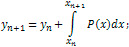
Thus, the Adams method allows us to account for significantly more information, resulting in more accurate results.
Newton’s Interpolation Polynomial: The Core Idea of the Adams Method
Where does this polynomial come from? It is based on Newton’s polynomial, which precisely approximates a function at several known points. The general form of Newton’s polynomial is:

This polynomial is easily constructed from the known values at previous points, and integrating it gives straightforward formulas for calculating the subsequent values of the function. That’s how different variants of the Adams method arise, depending on the number of points we use.
Adams Method Formulas for Different Numbers of Points: A Brief Overview
To see how this approach works in practice, let’s consider a few simple examples:
- Euler’s Method (j=0): uses only one point; the formula is simple.
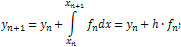
- Two-step Adams Method (j=1): considers two points; the formula is more accurate.

- Three-step Adams Method (j=2): considers three points; results are even better.

- Four-step Adams-Bashforth Method (j=3): four points provide extremely high accuracy.

As you can see, the more points we consider, the better results we obtain.
Why Adams Method Is an Excellent Choice?
The Adams method combines simplicity, speed, and accuracy. Its benefits are clear:
- High accuracy of results due to the use of more information.
- Computational speed—no need for many steps to achieve accurate solutions.
- Ease of implementation in computer programs, making this method accessible for students.
Thus, the Adams method is more than just another numerical method. It’s a powerful tool that significantly simplifies your work with differential equations and helps you quickly obtain reliable results.
Practical Application of the Numerical Method: Step-by-Step Problem Analysis
Now that we’ve covered the theory, it’s time to see exactly how the Adams method is used in practical problems. After all, it’s one thing to read formulas and quite another to see how they actually work. To better understand this, let’s examine a specific problem and carefully go through each step of its solution.
Example 1: Consider the Differential Equation y’=y-x With the Initial Condition y(0)=1.5. Our Goal is to Find an Approximate Solution For This Equation on the Interval [0, 1], and Then Compare These Approximate Results With the Exact Solution Given By the Formula: y(x)=0.5⋅ex+x+1

Since the Adams method is a multi-step method, we need initial points to start the calculation. How do we get them? The easiest way is to use the fourth-order Runge-Kutta method, which quickly provides accurate initial values.
First, we divide the interval [0,1] into 8 equal segments. Thus, our step size will be h=0.125. Therefore, we obtain the following points:

We can quickly find the initial four function values using an online Runge-Kutta calculator. By entering our equation and initial conditions, we get these results:

Now, having these initial values, we apply the fourth-order Adams-Bashforth method for subsequent points:

So, we’ve found approximate function values using the Adams method. Now let’s compare them with the exact values and calculate the errors:
| x | Approximate y | Exact y | Error |
|---|---|---|---|
| 0.5 | 2.33796 | 2.32436 | 0.0136 |
| 0.625 | 2.57661 | 2.55912 | 0.01749 |
| 0.75 | 2.82681 | 2.8085 | 0.01831 |
| 0.875 | 3.093 | 3.07444 | 0.01856 |
| 1 | 3.38011 | 3.35914 | 0.02097 |
As you can see, the results obtained using the Adams method are very close to the exact values. This is an excellent outcome considering that we’ve completed only eight steps. If we choose a smaller step size, the accuracy will become even greater!
Thus, the Adams method is not only theoretically sound for numerical problem solving but also a practically effective tool that allows you to easily obtain reliable results even for complex tasks.
Want to Learn More? Other Interesting Numerical Methods for Solving Differential Equations
The Adams method is indeed one of the most effective approaches to numerically solving differential equations. However, there are many other equally interesting and useful methods. If you found this topic intriguing and want to dive deeper, we recommend exploring these numerical methods:
- Milne’s Method – This multi-step method allows predicting solutions, then refining them using special correction formulas for high accuracy.
- Modified Euler’s Method – This is an improved version of the classical method, considering the average values of the function between points to achieve greater accuracy with minimal effort.
- Runge-Kutta-Merson Method – One of the most accurate numerical methods, automatically controlling accuracy by adjusting the integration step size during calculations.
Each of these methods has unique features, so you’ll easily find the best fit for any of your problems!
Turning Math into Code: Creating Your Own Solution
Understanding numerical methods opens exciting opportunities not only in mathematics but also in programming. Now that you’ve thoroughly grasped how the Adams method works, it’s time to transform your knowledge into something practical and beneficial! You can choose any programming language that suits you best: Python, Java, C++, or even JavaScript—the key is to find it comfortable and interesting.
To simplify creating your own program, use the flowchart below. It illustrates the Adams method logic step by step, making it easier to quickly write working code. So go ahead, experiment, and enjoy the process of developing your very own solution!
