A cubic spline is used to approximate a function whose values are known only at certain points. Instead of using a single high-degree polynomial, the entire interval is divided into smaller parts. A separate cubic polynomial is constructed between each pair of neighboring nodes, and these polynomials are joined to form one continuous and smooth curve. After looking at the main steps of spline construction, we will apply the resulting formulas to examples and find approximate function values from tabulated data.
Cubic Spline Interpolation: Moving from a Single Polynomial to a Piecewise Polynomial Approximation
Suppose a function is given at the points
\[
(x_0,y_0),\ (x_1,y_1),\ \dots,\ (x_n,y_n),
\]
where
\[
x_0<x_1<\dots<x_n.
\]
To approximate the function between the nodes, we can construct a single interpolating polynomial that passes through all the given points. This approach is used, for example, in the Lagrange and Newton interpolation formulas.
However, as the number of nodes increases, the degree of such a polynomial also increases. As a result, noticeable oscillations may appear between the nodes, especially near the ends of the interval. To avoid this problem, several low-degree polynomials are used instead of one high-degree polynomial.
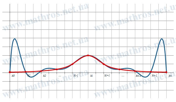
The entire interval
\[
[x_0,x_n]
\]
is divided into parts
\[
[x_0,x_1],\ [x_1,x_2],\ \dots,\ [x_{n-1},x_n].
\]
On each interval
\[
[x_i,x_{i+1}]
\]
a separate cubic polynomial is constructed:
\[
S_i(x)=a_i+b_i\cdot(x-x_i)+c_i\cdot(x-x_i)^2+d_i\cdot(x-x_i)^3,\qquad i=0,1,\dots,n-1.
\]
If \( n+1 \) nodes are given, they form \( n \) intervals, so \( n \) cubic polynomials must be constructed.
For further calculations, let us introduce the length of each interval:
\[
h_i=x_{i+1}-x_i,\qquad i=0,1,\dots,n-1.
\]
Each of the constructed polynomials describes the spline only on its own interval. To make all these parts form a single curve, they must be joined correctly at the nodes.
Cubic Spline: Conditions for Smoothly Joining the Polynomials
First of all, the spline must pass through all the given tabulated points. For each interval, the following conditions must be satisfied:
\[
S_i(x_i)=y_i,\qquad S_i(x_{i+1})=y_{i+1}.
\]
At the left node, we have
\[
S_i(x_i)=a_i,
\]
so
\[
a_i=y_i.
\]
Therefore, the coefficients \( a_i \) are determined directly from the tabulated function values.
At the right node,
\[
x_{i+1}-x_i=h_i,
\]
so
\[
a_i+b_i\cdot h_i+c_i\cdot h_i^2+d_i\cdot h_i^3=y_{i+1}.
\]
Passing through the nodes ensures that there are no breaks between neighboring parts of the spline. However, this alone is not enough to obtain a smooth curve.
Let us find the first derivative of the cubic polynomial:
\[
S_i'(x)=b_i+2\cdot c_i\cdot(x-x_i)+3\cdot d_i\cdot(x-x_i)^2.
\]
At each interior node, the following condition must be satisfied:
\[
S_{i-1}'(x_i)=S_i'(x_i),\qquad i=1,2,\dots,n-1.
\]
Equality of the first derivatives ensures that neighboring parts of the curve have the same slope at the node and prevents sharp corners from appearing.
The second derivative has the form
\[
S_i”(x)=2\cdot c_i+6\cdot d_i\cdot(x-x_i).
\]
To ensure a smooth change in curvature, the following additional condition is required at each interior node:
\[
S_{i-1}”(x_i)=S_i”(x_i),\qquad i=1,2,\dots,n-1.
\]
Thus, continuity of the function values eliminates breaks, continuity of the first derivative prevents sharp corners, and continuity of the second derivative ensures a smooth change in curvature.
To determine all the spline coefficients uniquely, we still need to specify the conditions at the endpoints of the entire interval.
Cubic Spline: Boundary Conditions and the Role of the Coefficients
In this article, we will use boundary conditions in which the second derivative of the spline is equal to zero at the first and last nodes:
\[
S”(x_0)=0,\qquad S”(x_n)=0.
\]
Let us look at how these conditions are related to the coefficients of the cubic polynomials.
At the left endpoint of the interval \( [x_i,x_{i+1}] \), we have
\[
S_i”(x_i)=2\cdot c_i.
\]
Therefore,
\[
c_i=\frac{S”(x_i)}{2}.
\]
Thus, the coefficients \( c_i \) are directly related to the second derivative of the spline at the nodes.
For the endpoint nodes, we have
\[
c_0=0,\qquad c_n=0.
\]
The coefficient \( c_n \) is related to the second derivative of the spline at the last node \( x_n \). There is no separate polynomial \( S_n(x) \), because the last polynomial is constructed on the interval \( [x_{n-1},x_n] \). However, the coefficient \( c_n \) is still needed to determine that polynomial.
At the right endpoint of any interval, we have
\[
S_i”(x_{i+1})=2\cdot c_i+6\cdot d_i\cdot h_i.
\]
On the other hand, the second derivative at the node \( x_{i+1} \) is determined by the coefficient \( c_{i+1} \), so
\[
2\cdot c_i+6\cdot d_i\cdot h_i=2\cdot c_{i+1}.
\]
Therefore,
\[
d_i=\frac{c_{i+1}-c_i}{3\cdot h_i},\qquad i=0,1,\dots,n-1.
\]
Now let us use the condition that the spline passes through the right node:
\[
a_i+b_i\cdot h_i+c_i\cdot h_i^2+d_i\cdot h_i^3=y_{i+1}.
\]
Since
\[
a_i=y_i,
\]
we obtain
\[
b_i=\frac{y_{i+1}-y_i}{h_i}-c_i\cdot h_i-d_i\cdot h_i^2.
\]
After substituting the formula for \( d_i \), we get
\[
b_i=\frac{y_{i+1}-y_i}{h_i}-\frac{h_i}{3}\cdot(2\cdot c_i+c_{i+1}),\qquad i=0,1,\dots,n-1.
\]
So, if the coefficients \( c_i \) are known, we can use them to find \( d_i \) and \( b_i \), while the coefficients \( a_i \) are already determined by the tabulated function values. Therefore, the main task is to find the interior coefficients \( c_i \).
Tridiagonal System: Determining the Cubic Spline Coefficients
To find the interior coefficients, we will use the continuity condition for the first derivative.
At the right endpoint of the interval \( [x_{i-1},x_i] \),
\[
S_{i-1}'(x_i)=b_{i-1}+2\cdot c_{i-1}\cdot h_{i-1}+3\cdot d_{i-1}\cdot h_{i-1}^2.
\]
At the left endpoint of the next interval,
\[
S_i'(x_i)=b_i.
\]
Therefore,
\[
b_{i-1}+2\cdot c_{i-1}\cdot h_{i-1}+3\cdot d_{i-1}\cdot h_{i-1}^2=b_i.
\]
Now substitute the formulas obtained earlier for \( b_{i-1} \), \( b_i \), and \( d_{i-1} \) into this equation. After simplification, only three neighboring coefficients remain:
\[
c_{i-1},\qquad c_i,\qquad c_{i+1}.
\]
For each interior node, we obtain the equation
\[
h_{i-1}\cdot c_{i-1}+2\cdot(h_{i-1}+h_i)\cdot c_i+h_i\cdot c_{i+1}
=
3\cdot\left(
\frac{y_{i+1}-y_i}{h_i}
–
\frac{y_i-y_{i-1}}{h_{i-1}}
\right),
\]
where
\[
i=1,2,\dots,n-1.
\]
Together with the boundary conditions
\[
c_0=0,\qquad c_n=0,
\]
we obtain a system for finding all the interior coefficients
\[
c_1,c_2,\dots,c_{n-1}.
\]
Each equation contains only three neighboring unknowns. Therefore, the system matrix has nonzero elements on the main diagonal and on the two diagonals directly next to it. Such a system is called a tridiagonal system, and the Thomas algorithm is a convenient method for solving it.
After finding the coefficients \( c_i \), we calculate \( d_i \) and \( b_i \), and then write down all the coefficients of the corresponding cubic polynomials. Next, a separate polynomial is constructed for each interval, and all these polynomials together form the cubic spline.
Cubic Spline: Step-by-Step Examples of Construction and Calculation
Let us move on to the practical use of a cubic spline for tabulated functions. In each case, we will find the required coefficients, determine the polynomial for the appropriate interval, and calculate an approximate value of the function.
Example 1. Using the given tabulated function values, find the approximate value of \( f(0.4) \)
| \( i \) | \( x_i \) | \( y_i \) |
|---|---|---|
| \( 0 \) | \( 0 \) | \( 1 \) |
| \( 1 \) | \( 1 \) | \( 2 \) |
| \( 2 \) | \( 2 \) | \( 5 \) |
We have three nodes and two intervals. Let us calculate their lengths:
\[
h_0=1-0=1,\qquad h_1=2-1=1.
\]
For the endpoint nodes, we have
\[
c_0=0,\qquad c_2=0.
\]
The only unknown coefficient is \( c_1 \). Let us write the equation for it:
\[
h_0\cdot c_0+2\cdot(h_0+h_1)\cdot c_1+h_1\cdot c_2
=
3\cdot\left(\frac{y_2-y_1}{h_1}-\frac{y_1-y_0}{h_0}\right).
\]
Substitute the values:
\[
1\cdot0+2\cdot(1+1)\cdot c_1+1\cdot0
=
3\cdot\left(\frac{5-2}{1}-\frac{2-1}{1}\right).
\]
We obtain
\[
4\cdot c_1=6,
\]
so
\[
c_1=1.5.
\]
Therefore,
\[
c_0=0,\qquad c_1=1.5,\qquad c_2=0.
\]
Now let us find the coefficients \( d_i \):
\[
\begin{gathered}
d_0=\frac{1.5-0}{3\cdot1}=0.5,\\[4pt]
d_1=\frac{0-1.5}{3\cdot1}=-0.5.
\end{gathered}
\]
Next, let us calculate the coefficients \( b_i \):
\[
\begin{gathered}
b_0=\frac{2-1}{1}-\frac{1}{3}\cdot(2\cdot0+1.5)=0.5,\\[4pt]
b_1=\frac{5-2}{1}-\frac{1}{3}\cdot(2\cdot1.5+0)=2.
\end{gathered}
\]
The coefficients \( a_i \) are
\[
a_0=1,\qquad a_1=2.
\]
For the first interval, we have
\[
S_0(x)=1+0.5\cdot x+0.5\cdot x^3.
\]
Since
\[
0<0.4<1,
\]
we use this polynomial:
\[
S_0(0.4)=1+0.5\cdot0.4+0.5\cdot0.4^3.
\]
This gives
\[
S_0(0.4)=1+0.2+0.032=1.232.
\]
Therefore,
\[
f(0.4)\approx1.232.
\]
Example 2. Using the given tabulated function values, find the approximate value of \( f(2.5) \)
| \( i \) | \( x_i \) | \( y_i \) |
|---|---|---|
| \( 0 \) | \( 0 \) | \( 0 \) |
| \( 1 \) | \( 2 \) | \( 2 \) |
| \( 2 \) | \( 3 \) | \( 4 \) |
| \( 3 \) | \( 5 \) | \( 6 \) |
The distances between neighboring nodes are different, so the values of \( h_i \) must be calculated separately for each interval:
\[
h_0=2,\qquad h_1=1,\qquad h_2=2.
\]
For the endpoint nodes, we have
\[
c_0=0,\qquad c_3=0.
\]
The unknown coefficients are \( c_1 \) and \( c_2 \).
For the first interior node, we have
\[
2\cdot0+2\cdot(2+1)\cdot c_1+c_2
=
3\cdot\left(\frac{4-2}{1}-\frac{2-0}{2}\right),
\]
which gives
\[
6\cdot c_1+c_2=3.
\]
For the second interior node,
\[
c_1+2\cdot(1+2)\cdot c_2+2\cdot0
=
3\cdot\left(\frac{6-4}{2}-\frac{4-2}{1}\right),
\]
so
\[
c_1+6\cdot c_2=-3.
\]
We obtain the system
\[
\begin{cases}
6\cdot c_1+c_2=3,\\
c_1+6\cdot c_2=-3.
\end{cases}
\]
Solving it, we find
\[
c_1=0.6,\qquad c_2=-0.6.
\]
Therefore,
\[
c_0=0,\qquad c_1=0.6,\qquad c_2=-0.6,\qquad c_3=0.
\]
Now let us find the coefficients \( d_i \):
\[
\begin{gathered}
d_0=\frac{0.6-0}{3\cdot2}=0.1,\\[4pt]
d_1=\frac{-0.6-0.6}{3\cdot1}=-0.4,\\[4pt]
d_2=\frac{0-(-0.6)}{3\cdot2}=0.1.
\end{gathered}
\]
Next, let us calculate the coefficients \( b_i \):
\[
\begin{gathered}
b_0=\frac{2-0}{2}-\frac{2}{3}\cdot(2\cdot0+0.6)=0.6,\\[4pt]
b_1=\frac{4-2}{1}-\frac{1}{3}\cdot(2\cdot0.6-0.6)=1.8,\\[4pt]
b_2=\frac{6-4}{2}-\frac{2}{3}\cdot(2\cdot(-0.6)+0)=1.8.
\end{gathered}
\]
The coefficients \( a_i \) are
\[
a_0=0,\qquad a_1=2,\qquad a_2=4.
\]
Since
\[
2<2.5<3,
\]
we need to use the polynomial on the interval \( [2,3] \):
\[
S_1(x)=2+1.8\cdot(x-2)+0.6\cdot(x-2)^2-0.4\cdot(x-2)^3.
\]
For \( x=2.5 \), we have
\[
S_1(2.5)=2+1.8\cdot0.5+0.6\cdot0.5^2-0.4\cdot0.5^3.
\]
This gives
\[
S_1(2.5)=2+0.9+0.15-0.05=3.
\]
Therefore,
\[
f(2.5)\approx3.
\]
Example 3. Using the given tabulated function values, find the approximate value of \( f(3.5) \)
| \( i \) | \( x_i \) | \( y_i \) |
|---|---|---|
| \( 0 \) | \( 0 \) | \( 0 \) |
| \( 1 \) | \( 1 \) | \( 2 \) |
| \( 2 \) | \( 2 \) | \( 7 \) |
| \( 3 \) | \( 3 \) | \( 10 \) |
| \( 4 \) | \( 4 \) | \( 16 \) |
In this case, all neighboring nodes are equally spaced:
\[
h_0=h_1=h_2=h_3=1.
\]
For the endpoint nodes, we have
\[
c_0=0,\qquad c_4=0.
\]
There are three interior nodes, so we need to write three equations for the coefficients \( c_1 \), \( c_2 \), and \( c_3 \).
For the first interior node,
\[
4\cdot c_1+c_2
=
3\cdot\left((7-2)-(2-0)\right),
\]
that is,
\[
4\cdot c_1+c_2=9.
\]
For the second interior node,
\[
c_1+4\cdot c_2+c_3
=
3\cdot\left((10-7)-(7-2)\right),
\]
which gives
\[
c_1+4\cdot c_2+c_3=-6.
\]
For the third interior node,
\[
c_2+4\cdot c_3
=
3\cdot\left((16-10)-(10-7)\right),
\]
so
\[
c_2+4\cdot c_3=9.
\]
We obtain the system
\[
\begin{cases}
4\cdot c_1+c_2=9,\\
c_1+4\cdot c_2+c_3=-6,\\
c_2+4\cdot c_3=9.
\end{cases}
\]
Solving it, we find
\[
c_1=3,\qquad c_2=-3,\qquad c_3=3.
\]
Therefore,
\[
c_0=0,\qquad c_1=3,\qquad c_2=-3,\qquad c_3=3,\qquad c_4=0.
\]
Now let us find the coefficients \( d_i \):
\[
d_0=1,\qquad d_1=-2,\qquad d_2=2,\qquad d_3=-1.
\]
Next, let us calculate the coefficients \( b_i \):
\[
b_0=1,\qquad b_1=4,\qquad b_2=4,\qquad b_3=4.
\]
The coefficients \( a_i \) are
\[
a_0=0,\qquad a_1=2,\qquad a_2=7,\qquad a_3=10.
\]
The given value \( x=3.5 \) lies in the last interval:
\[
3<3.5<4.
\]
Therefore, we use the polynomial
\[
S_3(x)=10+4\cdot(x-3)+3\cdot(x-3)^2-(x-3)^3.
\]
For \( x=3.5 \), we have
\[
S_3(3.5)=10+4\cdot0.5+3\cdot0.5^2-0.5^3.
\]
This gives
\[
S_3(3.5)=10+2+0.75-0.125=12.625.
\]
Therefore,
\[
f(3.5)\approx12.625.
\]
Next Topics: Continue Exploring Interpolation
A cubic spline shows how to build a smooth approximation from tabulated data, but interpolation also offers other interesting approaches. Next, it is worth exploring methods designed for periodic functions and for interpolation near the middle of a table.
- Trigonometric Interpolation: Approximation of Periodic Functions — We will look at how to construct approximations of periodic functions from tabulated values using sines and cosines.
- Gauss Interpolation Formulas: Calculating Values Near the Middle of a Table — We will learn how Gauss’s first and second interpolation formulas can be used to find approximate function values near the central nodes of a table.
- Bessel’s Formula: Interpolation Between the Central Nodes of a Table — We will explore how Bessel’s formula helps calculate approximate function values when the value of \( x \) lies between the central nodes.
Cubic Spline: Turn the Algorithm into Your Own Program
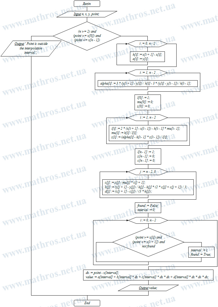
If you enjoy programming, try putting what you have learned into practice by implementing the cubic spline construction algorithm yourself. Use the given flowchart as a guide: enter the nodes and function values, calculate the spline coefficients, determine the interval containing the given point, and find the approximate function value. Choose the programming language you feel most comfortable working with — Pascal, Python, C++, JavaScript, or any other language.