The Lagrange interpolation polynomial makes it possible to construct a polynomial approximation of a function from its known values at given interpolation nodes. At the nodes themselves, the polynomial values exactly match the given function values, while between the nodes, the polynomial is used to approximate the function. Let us look at how this polynomial is constructed for unequally spaced nodes and then apply the resulting formula to practical examples.
Unequally Spaced Interpolation Nodes: Conditions and Problem Statement
Suppose that \( n+1 \) pairwise distinct and ordered interpolation nodes are given on the interval \( [a,b] \):
\[
a\leq x_0<x_1<\dots<x_n\leq b.
\]
For each node, the corresponding function value is known:
\[
f(x_0)=y_0,\quad f(x_1)=y_1,\quad\dots,\quad f(x_n)=y_n.
\]
Let the distance between two neighboring nodes be denoted by
\[
h_i=x_{i+1}-x_i,\qquad i=0,1,\dots,n-1.
\]
If the values \( h_i \) are not the same for all \( i \), the nodes are called unequally spaced.
The task is to construct a polynomial \( L_n(x) \) of degree at most \( n \) that takes the corresponding given function value at each interpolation node:
\[
L_n(x_i)=y_i,\qquad i=0,1,2,\dots,n.
\]
Thus, the graph of the required polynomial passes through all the given points
\[
(x_0,y_0),\quad(x_1,y_1),\quad\dots,\quad(x_n,y_n).
\]
For \( n+1 \) pairwise distinct nodes, there exists a unique polynomial of degree at most \( n \) that satisfies these interpolation conditions. To construct it, we will use the Lagrange basis polynomials.
Lagrange Interpolation Polynomial: Construction Using Basis Polynomials
We represent the polynomial \( L_n(x) \) as a linear combination of the known function values at the interpolation nodes:
\[
L_n(x)=\sum_{i=0}^{n}P_i(x)\cdot y_i,
\]
where \( P_i(x) \) are the Lagrange basis polynomials.
Each basis polynomial \( P_i(x) \) is constructed so that it equals \( 1 \) at the node \( x_i \) and \( 0 \) at all the other nodes:
\[
P_i(x_j)=\begin{cases}1, & i=j,\\0, & i\neq j.\end{cases}
\]
Let us substitute one of the nodes \( x_i \) into the polynomial \( L_n(x) \):
\[
L_n(x_i)=P_0(x_i)\cdot y_0+\dots+P_i(x_i)\cdot y_i+\dots+P_n(x_i)\cdot y_n=y_i.
\]
All terms for which the index of the basis polynomial does not match the index of the node are equal to zero. Only the term \( P_i(x_i)\cdot y_i=y_i \) remains, so the constructed polynomial takes the required value at every interpolation node.
To ensure that \( P_i(x_j)=0 \) when \( j\neq i \), the basis polynomial includes factors that become zero at the corresponding nodes:
\[
P_i(x)=c_i\cdot(x-x_0)\cdot(x-x_1)\cdot\dots\cdot(x-x_{i-1})\cdot(x-x_{i+1})\cdot\dots\cdot(x-x_n),
\]
where \( c_i \) is a constant coefficient.
The factor \( x-x_i \) is not included in this product, so when \( x=x_i \), the basis polynomial does not become zero. We find the value of the coefficient \( c_i \) from the condition
\[
P_i(x_i)=1.
\]
Substituting \( x=x_i \), we obtain
\[
c_i\cdot(x_i-x_0)\cdot(x_i-x_1)\cdot\dots\cdot(x_i-x_{i-1})\cdot(x_i-x_{i+1})\cdot\dots\cdot(x_i-x_n)=1.
\]
Therefore,
\[
c_i=\frac{1}{(x_i-x_0)\cdot(x_i-x_1)\cdot\dots\cdot(x_i-x_{i-1})\cdot(x_i-x_{i+1})\cdot\dots\cdot(x_i-x_n)}.
\]
Now substitute the coefficient we found into the expression for \( P_i(x) \). This gives the Lagrange basis polynomial:
\[
P_i(x)=\frac{(x-x_0)\cdot(x-x_1)\cdot\dots\cdot(x-x_{i-1})\cdot(x-x_{i+1})\cdot\dots\cdot(x-x_n)}{(x_i-x_0)\cdot(x_i-x_1)\cdot\dots\cdot(x_i-x_{i-1})\cdot(x_i-x_{i+1})\cdot\dots\cdot(x_i-x_n)}.
\]
Since the nodes \( x_0,x_1,\dots,x_n \) are pairwise distinct, for \( i\neq j \) we have
\[
x_i-x_j\neq0.
\]
Therefore, none of the factors in the denominator of the basis polynomial is equal to zero.
Now substitute this expression for \( P_i(x) \) into the formula for \( L_n(x) \). As a result, we obtain the general form of the Lagrange interpolation polynomial:
\[
L_n(x)=\sum_{i=0}^{n}\frac{(x-x_0)\cdot(x-x_1)\cdot\dots\cdot(x-x_{i-1})\cdot(x-x_{i+1})\cdot\dots\cdot(x-x_n)}{(x_i-x_0)\cdot(x_i-x_1)\cdot\dots\cdot(x_i-x_{i-1})\cdot(x_i-x_{i+1})\cdot\dots\cdot(x_i-x_n)}\cdot y_i.
\]
After the basis polynomials \( P_i(x) \) have been constructed, their values together with the tabulated values \( y_i \) can be used directly to calculate \( L_n(x) \) at a given point.
Lagrange Interpolation Polynomial: Practical Application
Let us see how to construct the basis polynomials step by step from given tabulated values and then calculate the value of the interpolation polynomial at a specified point. We will start with three nodes and then increase their number to four and five.
Example 1. Using the given tabulated function values, find the approximate value of \( f(1.5) \)
| \( i \) | \( x_i \) | \( y_i \) |
|---|---|---|
| \( 0 \) | \( 1 \) | \( 1 \) |
| \( 1 \) | \( 2 \) | \( 4 \) |
| \( 2 \) | \( 4 \) | \( 16 \) |
The distances between neighboring nodes are
\[
h_0=x_1-x_0=1,\qquad h_1=x_2-x_1=2.
\]
Since \( h_0\neq h_1 \), the nodes are unequally spaced.
For three nodes, the Lagrange interpolation polynomial has the form
\[
L_2(x)=P_0(x)\cdot y_0+P_1(x)\cdot y_1+P_2(x)\cdot y_2.
\]
Let us construct the first basis polynomial:
\[
P_0(x)=\frac{(x-x_1)\cdot(x-x_2)}{(x_0-x_1)\cdot(x_0-x_2)}.
\]
For \( x=1.5 \), we obtain
\[
P_0(1.5)=\frac{(1.5-2)\cdot(1.5-4)}{(1-2)\cdot(1-4)}=\frac{5}{12}\approx0.417.
\]
The second basis polynomial has the form
\[
P_1(x)=\frac{(x-x_0)\cdot(x-x_2)}{(x_1-x_0)\cdot(x_1-x_2)}.
\]
Then
\[
P_1(1.5)=\frac{(1.5-1)\cdot(1.5-4)}{(2-1)\cdot(2-4)}=\frac{5}{8}\approx0.625.
\]
For the third basis polynomial, we have
\[
P_2(x)=\frac{(x-x_0)\cdot(x-x_1)}{(x_2-x_0)\cdot(x_2-x_1)}.
\]
Substituting \( x=1.5 \), we obtain
\[
P_2(1.5)=\frac{(1.5-1)\cdot(1.5-2)}{(4-1)\cdot(4-2)}=-\frac{1}{24}\approx-0.042.
\]
Now substitute the calculated values of the basis polynomials:
\[
L_2(1.5)=\frac{5}{12}\cdot1+\frac{5}{8}\cdot4-\frac{1}{24}\cdot16\approx2.25.
\]
Therefore,
\[
f(1.5)\approx2.25.
\]
Example 2. Using the given tabulated function values, find the approximate value of \( f(2) \)
| \( i \) | \( x_i \) | \( y_i \) |
|---|---|---|
| \( 0 \) | \( 0 \) | \( 0 \) |
| \( 1 \) | \( 1 \) | \( 1 \) |
| \( 2 \) | \( 3 \) | \( 27 \) |
| \( 3 \) | \( 4 \) | \( 64 \) |
The distances between neighboring nodes are
\[
h_0=1,\qquad h_1=2,\qquad h_2=1.
\]
The nodes are unequally spaced.
For four nodes, the Lagrange interpolation polynomial has the form
\[
L_3(x)=P_0(x)\cdot y_0+P_1(x)\cdot y_1+P_2(x)\cdot y_2+P_3(x)\cdot y_3.
\]
Let us construct the first basis polynomial:
\[
P_0(x)=\frac{(x-x_1)\cdot(x-x_2)\cdot(x-x_3)}{(x_0-x_1)\cdot(x_0-x_2)\cdot(x_0-x_3)}.
\]
For \( x=2 \), we obtain
\[
P_0(2)=\frac{(2-1)\cdot(2-3)\cdot(2-4)}{(0-1)\cdot(0-3)\cdot(0-4)}=-\frac{1}{6}\approx-0.167.
\]
The second basis polynomial has the form
\[
P_1(x)=\frac{(x-x_0)\cdot(x-x_2)\cdot(x-x_3)}{(x_1-x_0)\cdot(x_1-x_2)\cdot(x_1-x_3)}.
\]
Then
\[
P_1(2)=\frac{(2-0)\cdot(2-3)\cdot(2-4)}{(1-0)\cdot(1-3)\cdot(1-4)}=\frac{2}{3}\approx0.667.
\]
The third basis polynomial has the form
\[
P_2(x)=\frac{(x-x_0)\cdot(x-x_1)\cdot(x-x_3)}{(x_2-x_0)\cdot(x_2-x_1)\cdot(x_2-x_3)}.
\]
Substituting \( x=2 \), we obtain
\[
P_2(2)=\frac{(2-0)\cdot(2-1)\cdot(2-4)}{(3-0)\cdot(3-1)\cdot(3-4)}=\frac{2}{3}\approx0.667.
\]
For the fourth basis polynomial, we have
\[
P_3(x)=\frac{(x-x_0)\cdot(x-x_1)\cdot(x-x_2)}{(x_3-x_0)\cdot(x_3-x_1)\cdot(x_3-x_2)}.
\]
Then
\[
P_3(2)=\frac{(2-0)\cdot(2-1)\cdot(2-3)}{(4-0)\cdot(4-1)\cdot(4-3)}=-\frac{1}{6}\approx-0.167.
\]
Now substitute the calculated values of the basis polynomials:
\[
L_3(2)=-\frac{1}{6}\cdot0+\frac{2}{3}\cdot1+\frac{2}{3}\cdot27-\frac{1}{6}\cdot64=8.
\]
Therefore,
\[
f(2)\approx8.
\]
Example 3. Using the given tabulated function values, find the approximate value of \( f(5.5) \)
| \( i \) | \( x_i \) | \( y_i \) |
|---|---|---|
| \( 0 \) | \( 0 \) | \( 0 \) |
| \( 1 \) | \( 1 \) | \( 1 \) |
| \( 2 \) | \( 3 \) | \( 81 \) |
| \( 3 \) | \( 5 \) | \( 625 \) |
| \( 4 \) | \( 6 \) | \( 1296 \) |
The distances between neighboring nodes are
\[
h_0=1,\qquad h_1=2,\qquad h_2=2,\qquad h_3=1.
\]
The nodes are unequally spaced.
For five nodes, the Lagrange interpolation polynomial has the form
\[
L_4(x)=P_0(x)\cdot y_0+P_1(x)\cdot y_1+P_2(x)\cdot y_2+P_3(x)\cdot y_3+P_4(x)\cdot y_4.
\]
Let us construct the first basis polynomial:
\[
P_0(x)=\frac{(x-x_1)\cdot(x-x_2)\cdot(x-x_3)\cdot(x-x_4)}{(x_0-x_1)\cdot(x_0-x_2)\cdot(x_0-x_3)\cdot(x_0-x_4)}.
\]
For \( x=5.5 \), we obtain
\[
P_0(5.5)=\frac{(5.5-1)\cdot(5.5-3)\cdot(5.5-5)\cdot(5.5-6)}{(0-1)\cdot(0-3)\cdot(0-5)\cdot(0-6)}=-\frac{1}{32}\approx-0.031.
\]
The second basis polynomial has the form
\[
P_1(x)=\frac{(x-x_0)\cdot(x-x_2)\cdot(x-x_3)\cdot(x-x_4)}{(x_1-x_0)\cdot(x_1-x_2)\cdot(x_1-x_3)\cdot(x_1-x_4)}.
\]
Then
\[
P_1(5.5)=\frac{(5.5-0)\cdot(5.5-3)\cdot(5.5-5)\cdot(5.5-6)}{(1-0)\cdot(1-3)\cdot(1-5)\cdot(1-6)}=\frac{11}{128}\approx0.086.
\]
The third basis polynomial has the form
\[
P_2(x)=\frac{(x-x_0)\cdot(x-x_1)\cdot(x-x_3)\cdot(x-x_4)}{(x_2-x_0)\cdot(x_2-x_1)\cdot(x_2-x_3)\cdot(x_2-x_4)}.
\]
For \( x=5.5 \), we have
\[
P_2(5.5)=\frac{(5.5-0)\cdot(5.5-1)\cdot(5.5-5)\cdot(5.5-6)}{(3-0)\cdot(3-1)\cdot(3-5)\cdot(3-6)}=-\frac{11}{64}\approx-0.172.
\]
For the fourth basis polynomial, we obtain
\[
P_3(x)=\frac{(x-x_0)\cdot(x-x_1)\cdot(x-x_2)\cdot(x-x_4)}{(x_3-x_0)\cdot(x_3-x_1)\cdot(x_3-x_2)\cdot(x_3-x_4)}.
\]
Then
\[
P_3(5.5)=\frac{(5.5-0)\cdot(5.5-1)\cdot(5.5-3)\cdot(5.5-6)}{(5-0)\cdot(5-1)\cdot(5-3)\cdot(5-6)}=\frac{99}{128}\approx0.773.
\]
The fifth basis polynomial has the form
\[
P_4(x)=\frac{(x-x_0)\cdot(x-x_1)\cdot(x-x_2)\cdot(x-x_3)}{(x_4-x_0)\cdot(x_4-x_1)\cdot(x_4-x_2)\cdot(x_4-x_3)}.
\]
Substituting \( x=5.5 \), we obtain
\[
P_4(5.5)=\frac{(5.5-0)\cdot(5.5-1)\cdot(5.5-3)\cdot(5.5-5)}{(6-0)\cdot(6-1)\cdot(6-3)\cdot(6-5)}=\frac{11}{32}\approx0.344.
\]
Now substitute the calculated values of the basis polynomials:
\[
L_4(5.5)=-\frac{1}{32}\cdot0+\frac{11}{128}\cdot1-\frac{11}{64}\cdot81+\frac{99}{128}\cdot625+\frac{11}{32}\cdot1296\approx915.063.
\]
Therefore,
\[
f(5.5)\approx915.063.
\]
What to Study Next: Topics for Further Study
After learning about the Lagrange interpolation polynomial, it is worth exploring other methods for approximating functions given by tabulated data. These methods will help you compare different approaches and understand which one is better suited to a particular problem.
- Least Squares Method: Function Approximation from Tabulated Data — Learn how to construct an approximate function from a set of data so that the total deviation of the calculated values from the given values is minimized.
- Linear Interpolation: Calculating Intermediate Function Values — See how two neighboring tabulated values can be used to quickly and easily estimate a function value within a given interval.
- Quadratic Interpolation: Function Approximation Using Three Nodes — Learn how a quadratic polynomial and three neighboring nodes can be used to estimate intermediate function values more accurately.
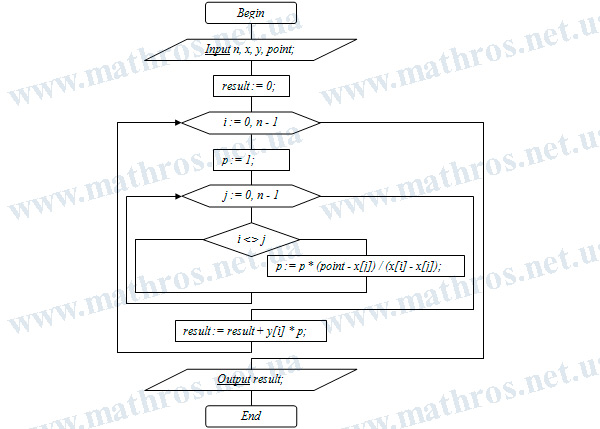
Lagrange Interpolation Polynomial: From Flowchart to Code
Do you enjoy programming? Then try turning your knowledge of the Lagrange interpolation polynomial into your own code. Use the flowchart below and implement the algorithm in whichever programming language you prefer—Pascal, Python, JavaScript, C++, or any other language.
The program should read the interpolation nodes, the corresponding function values, and the specified point, and then calculate the approximate function value using the Lagrange formula. This way, you can not only test how the method works with different data sets but also see how a sequence of mathematical calculations is transformed into code.