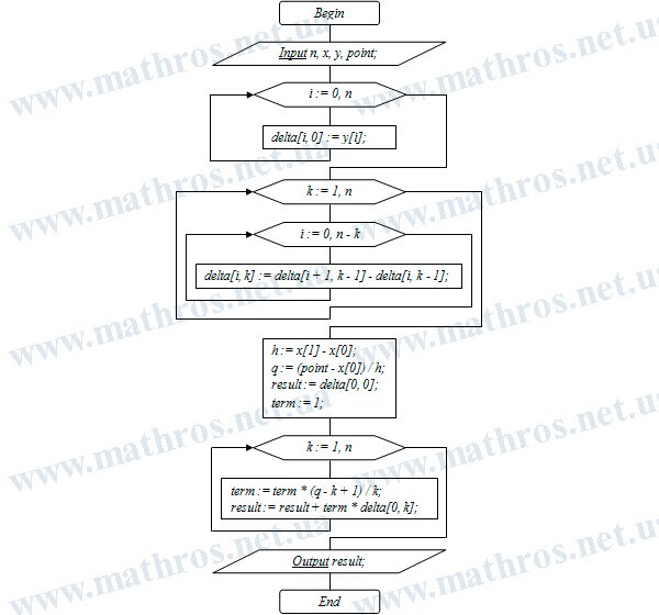
Newton’s forward interpolation formula makes it possible to approximate function values from tabulated data at equally spaced points. In this article, we will learn how to construct a forward finite difference table, build an interpolation polynomial, and rewrite it in a form that is convenient for calculations. Step-by-step examples will help you understand how to apply the formula in practice.
Newton’s Forward Interpolation Formula: Formulating the Interpolation Problem
Suppose that the values of the function \( y=f(x) \) are known:
\[ y_i=f(x_i), \qquad i=0,1,2,\dots,n, \]
at equally spaced interpolation points:
\[ x_i=x_0+i\cdot h, \]
where \( h\neq 0 \) is the constant spacing between consecutive interpolation points.
For \( n+1 \) distinct points, there is a unique polynomial \( P_n(x) \) whose degree does not exceed \( n \) and which satisfies the interpolation conditions
\[ P_n(x_i)=y_i, \qquad i=0,1,2,\dots,n. \]
At the interpolation points, the polynomial values exactly match the given function values. At other points, the polynomial is used to approximate the function values.
We will look for Newton’s interpolation polynomial in the following form:
\[ P_n(x)=a_0+a_1\cdot(x-x_0)+a_2\cdot(x-x_0)\cdot(x-x_1)+\dots+a_n\cdot(x-x_0)\cdot(x-x_1)\cdot\dots\cdot(x-x_{n-1}), \]
where \( a_0,a_1,\dots,a_n \) are unknown coefficients.
Each new term contains one additional factor. This structure allows us to determine the coefficients one by one, starting with \( a_0 \).
To simplify the notation, let us introduce
\[ \begin{gathered} (x-x_0)^{[0]}=1,\\[4pt] \qquad (x-x_0)^{[k]}=(x-x_0)\cdot(x-x_1)\cdot\dots\cdot(x-x_{k-1}), \qquad k\geq 1. \end{gathered} \]
This product of consecutive factors is called a generalized power. Using this notation, the polynomial can be written more compactly:
\[ P_n(x)=a_0+a_1\cdot(x-x_0)^{[1]}+a_2\cdot(x-x_0)^{[2]}+\dots+a_n\cdot(x-x_0)^{[n]}. \]
A generalized power should not be confused with an ordinary power. For example,
\[ (x-x_0)^{[2]}=(x-x_0)\cdot(x-x_1), \]
whereas
\[ (x-x_0)^2=(x-x_0)\cdot(x-x_0). \]
Therefore, these expressions have different structures and, in most cases, different values.
Forward Finite Differences: Constructing the Difference Table
Since the interpolation points are equally spaced, it is convenient to express the polynomial coefficients using forward finite differences.
A forward finite difference shows how the value of a function changes when moving from a point \( x \) to the next point \( x+h \). For an arbitrary function \( g(x) \), it is defined as
\[ \Delta g(x)=g(x+h)-g(x). \]
If \( x=x_i \), then
\[ x_i+h=x_{i+1}. \]
Therefore, a forward finite difference compares the function values at two consecutive interpolation points.
For tabulated function values, the first-order difference is
\[ \Delta y_i=y_{i+1}-y_i. \]
In particular,
\[ \Delta y_0=y_1-y_0, \qquad \Delta y_1=y_2-y_1, \qquad \Delta y_2=y_3-y_2. \]
Second-order differences are calculated from first-order differences:
\[ \Delta^2y_i=\Delta y_{i+1}-\Delta y_i. \]
For example,
\[ \Delta^2y_0=\Delta y_1-\Delta y_0, \qquad \Delta^2y_1=\Delta y_2-\Delta y_1. \]
In general, a finite difference of order \( k \) is defined recursively:
\[ \Delta^ky_i=\Delta^{k-1}y_{i+1}-\Delta^{k-1}y_i. \]
Each new order of differences is formed from the previous one. For \( n+1 \) given function values, finite differences can be calculated up to and including order \( n \).
Newton’s forward interpolation formula uses the initial function value and the differences of each order calculated from the beginning of the table:
\[ y_0,\qquad \Delta y_0,\qquad \Delta^2y_0,\qquad \dots,\qquad \Delta^ny_0. \]
The calculation starts at \( x_0 \) and proceeds toward points with higher indices. For this reason, Newton’s first interpolation formula is also known as Newton’s forward interpolation formula, or simply Newton’s forward formula.
Polynomial Coefficients: Step-by-Step Derivation
First, let us find the coefficient \( a_0 \). To do this, substitute \( x=x_0 \) into the polynomial. Every term except the first contains the factor \( x-x_0 \), so all these terms are equal to zero:
\[ P_n(x_0)=a_0. \]
According to the interpolation condition,
\[ P_n(x_0)=y_0. \]
Therefore,
\[ a_0=y_0. \]
Now apply the definition of the forward finite difference to the polynomial \( P_n(x) \):
\[ \Delta P_n(x)=P_n(x+h)-P_n(x). \]
For a generalized power, the following relation holds:
\[ \Delta(x-x_0)^{[k]}=k\cdot h\cdot(x-x_0)^{[k-1]}. \]
After calculating the first finite difference and substituting \( x=x_0 \), the term containing \( a_1 \) becomes \( a_1\cdot h \). All the remaining terms contain generalized powers of positive order, which are equal to zero at \( x_0 \). Therefore,
\[ \Delta P_n(x_0)=a_1\cdot h. \]
On the other hand,
\[ \Delta P_n(x_0)=P_n(x_0+h)-P_n(x_0). \]
Since
\[ x_1=x_0+h, \]
we obtain
\[ \Delta P_n(x_0)=P_n(x_1)-P_n(x_0). \]
At the interpolation points, the polynomial values match the function values. Therefore,
\[ \Delta P_n(x_0)=y_1-y_0=\Delta y_0. \]
Hence,
\[ a_1=\frac{\Delta y_0}{h}. \]
To determine the coefficient \( a_2 \), calculate the second-order finite difference. After substituting \( x=x_0 \), we obtain
\[ \Delta^2P_n(x_0)=2!\cdot a_2\cdot h^2. \]
Since
\[ \Delta^2P_n(x_0)=\Delta^2y_0, \]
it follows that
\[ a_2=\frac{\Delta^2y_0}{2!\cdot h^2}. \]
Each application of the finite-difference operator reduces the order of the generalized power by one and introduces the corresponding numerical factor and an additional factor \( h \). Therefore, after calculating the finite difference of order \( k \), we have
\[ \Delta^kP_n(x_0)=k!\cdot a_k\cdot h^k. \]
Hence,
\[ a_k=\frac{\Delta^ky_0}{k!\cdot h^k}, \qquad k=1,2,\dots,n. \]
Substituting the coefficients into the polynomial gives
\[ P_n(x)=y_0+\frac{\Delta y_0}{1!\cdot h}\cdot(x-x_0)^{[1]}+\frac{\Delta^2y_0}{2!\cdot h^2}\cdot(x-x_0)^{[2]}+\dots+\frac{\Delta^ny_0}{n!\cdot h^n}\cdot(x-x_0)^{[n]}. \]
Normalized Variable: Simplifying the Formula
To simplify the calculations, introduce the variable
\[ q=\frac{x-x_0}{h}. \]
It follows that
\[ x-x_0=q\cdot h. \]
Since
\[ x_j=x_0+j\cdot h, \]
we have
\[ x-x_j=x-x_0-j\cdot h=q\cdot h-j\cdot h=(q-j)\cdot h. \]
Therefore, the generalized power can be written as
\[ (x-x_0)^{[k]}=h^k\cdot q\cdot(q-1)\cdot(q-2)\cdot\dots\cdot(q-k+1). \]
Let us consider this transformation for the second-order term:
\[ \frac{\Delta^2y_0}{2!\cdot h^2}\cdot h^2\cdot q\cdot(q-1)=\frac{q\cdot(q-1)}{2!}\cdot\Delta^2y_0. \]
The factor \( h^2 \) that appears in this product cancels with the same factor in the denominator of the coefficient. The same cancellation occurs in all the following terms.
As a result, we obtain Newton’s forward interpolation formula:
\[ P_n(x)=y_0+q\cdot\Delta y_0+\frac{q\cdot(q-1)}{2!}\cdot\Delta^2y_0+\frac{q\cdot(q-1)\cdot(q-2)}{3!}\cdot\Delta^3y_0+\dots+\frac{q\cdot(q-1)\cdot(q-2)\cdot\dots\cdot(q-n+1)}{n!}\cdot\Delta^ny_0. \]
The variable \( q \) shows how far the point \( x \) is from the initial interpolation point \( x_0 \), measured in units of the step \( h \). Its value does not have to be an integer. For example, \( q=1.5 \) means that the point \( x \) is one and a half steps from \( x_0 \).
Newton’s forward interpolation formula is most convenient when the point \( x \) is located near the initial interpolation point \( x_0 \).
Newton’s Forward Interpolation Formula: Step-by-Step Examples
Let us now apply the formula to tabulated data with equally spaced interpolation points. In the first example, we will examine every calculation step in detail. Then we will see how the solution changes as the number of points and the order of the finite differences increase.
Example 1. Use the given tabulated function values to approximate \( f(1.5) \)
| \( i \) | \( x_i \) | \( y_i \) |
|---|---|---|
| \( 0 \) | \( 1 \) | \( 1 \) |
| \( 1 \) | \( 2 \) | \( 4 \) |
| \( 2 \) | \( 3 \) | \( 9 \) |
The interpolation points are equally spaced. The interpolation step is
\[ h=x_1-x_0=2-1=1. \]
Calculate the first-order finite differences:
\[ \Delta y_0=y_1-y_0=4-1=3, \qquad \Delta y_1=y_2-y_1=9-4=5. \]
Now find the second-order finite difference:
\[ \Delta^2y_0=\Delta y_1-\Delta y_0=5-3=2. \]
The calculated values can be arranged in a finite difference table.
| \( i \) | \( x_i \) | \( y_i \) | \( \Delta y_i \) | \( \Delta^2y_i \) |
|---|---|---|---|---|
| \( 0 \) | \( 1 \) | \( 1 \) | \( 3 \) | \( 2 \) |
| \( 1 \) | \( 2 \) | \( 4 \) | \( 5 \) | — |
| \( 2 \) | \( 3 \) | \( 9 \) | — | — |
Calculate the value of \( q \):
\[ q=\frac{x-x_0}{h}=\frac{1.5-1}{1}=0.5. \]
For three interpolation points, we use the formula
\[ P_2(x)=y_0+q\cdot\Delta y_0+\frac{q\cdot(q-1)}{2!}\cdot\Delta^2y_0. \]
Substitute the calculated values:
\[ P_2(1.5)=1+0.5\cdot3+\frac{0.5\cdot(0.5-1)}{2!}\cdot2. \]
Perform the calculations:
\[ P_2(1.5)=1+1.5-0.25=2.25. \]
Therefore,
\[ f(1.5)\approx2.25. \]
Example 2. Use the given tabulated function values to approximate \( f(1.2) \)
| \( i \) | \( x_i \) | \( y_i \) |
|---|---|---|
| \( 0 \) | \( 1 \) | \( 5 \) |
| \( 1 \) | \( 1.5 \) | \( 8.375 \) |
| \( 2 \) | \( 2 \) | \( 4 \) |
| \( 3 \) | \( 2.5 \) | \( 22.625 \) |
The step between two consecutive interpolation points is
\[ h=x_1-x_0=1.5-1=0.5. \]
Calculate the finite differences step by step up to the third order:
\[ \begin{gathered} \Delta y_0=8.375-5=3.375, \qquad \Delta y_1=14-8.375=5.625, \qquad \Delta y_2=22.625-14=8.625,\\[4pt] \Delta^2y_0=5.625-3.375=2.25, \qquad \Delta^2y_1=8.625-5.625=3,\\[4pt] \Delta^3y_0=3-2.25=0.75. \end{gathered} \]
Write the results in a finite difference table.
| \( i \) | \( x_i \) | \( y_i \) | \( \Delta y_i \) | \( \Delta^2y_i \) | \( \Delta^3y_i \) |
|---|---|---|---|---|---|
| \( 0 \) | \( 1 \) | \( 5 \) | \( 3.375 \) | \( 2.25 \) | \( 0.75 \) |
| \( 1 \) | \( 1.5 \) | \( 8.375 \) | \( 5.625 \) | \( 3 \) | — |
| \( 2 \) | \( 2 \) | \( 14 \) | \( 8.625 \) | — | — |
| \( 3 \) | \( 2.5 \) | \( 22.625 \) | — | — | — |
Calculate the value of \( q \):
\[ q=\frac{x-x_0}{h}=\frac{1.2-1}{0.5}=0.4. \]
For four interpolation points, we have
\[ P_3(x)=y_0+q\cdot\Delta y_0+\frac{q\cdot(q-1)}{2!}\cdot\Delta^2y_0+\frac{q\cdot(q-1)\cdot(q-2)}{3!}\cdot\Delta^3y_0. \]
Substitute the known values:
\[ P_3(1.2)=5+0.4\cdot3.375+\frac{0.4\cdot(0.4-1)}{2!}\cdot2.25+\frac{0.4\cdot(0.4-1)\cdot(0.4-2)}{3!}\cdot0.75. \]
Calculate the individual terms:
\[ \begin{gathered} 0.4\cdot3.375=1.35,\\[4pt] \frac{0.4\cdot(0.4-1)}{2!}\cdot2.25=-0.27,\\[4pt] \frac{0.4\cdot(0.4-1)\cdot(0.4-2)}{3!}\cdot0.75=0.048. \end{gathered} \]
Therefore,
\[ P_3(1.2)=5+1.35-0.27+0.048=6.128. \]
Thus,
\[ f(1.2)\approx6.128. \]
Example 3. Use the given tabulated function values to approximate \( f(1.6) \)
| \( i \) | \( x_i \) | \( y_i \) |
|---|---|---|
| \( 0 \) | \( 0 \) | \( 2 \) |
| \( 1 \) | \( 2 \) | \( 2 \) |
| \( 2 \) | \( 4 \) | \( 12 \) |
| \( 3 \) | \( 6 \) | \( 68 \) |
| \( 4 \) | \( 8 \) | \( 230 \) |
The interpolation step is
\[ h=x_1-x_0=2-0=2. \]
Using the tabulated values, calculate the finite differences step by step up to the fourth order:
\[ \begin{gathered} \Delta y_0=2-2=0, \qquad \Delta y_1=12-2=10, \qquad \Delta y_2=68-12=56, \qquad \Delta y_3=230-68=162,\\[4pt] \Delta^2y_0=10-0=10, \qquad \Delta^2y_1=56-10=46, \qquad \Delta^2y_2=162-56=106,\\[4pt] \Delta^3y_0=46-10=36, \qquad \Delta^3y_1=106-46=60,\\[4pt] \Delta^4y_0=60-36=24. \end{gathered} \]
Arrange the results in a finite difference table.
| \( i \) | \( x_i \) | \( y_i \) | \( \Delta y_i \) | \( \Delta^2y_i \) | \( \Delta^3y_i \) | \( \Delta^4y_i \) |
|---|---|---|---|---|---|---|
| \( 0 \) | \( 0 \) | \( 2 \) | \( 0 \) | \( 10 \) | \( 36 \) | \( 24 \) |
| \( 1 \) | \( 2 \) | \( 2 \) | \( 10 \) | \( 46 \) | \( 60 \) | — |
| \( 2 \) | \( 4 \) | \( 12 \) | \( 56 \) | \( 106 \) | — | — |
| \( 3 \) | \( 6 \) | \( 68 \) | \( 162 \) | — | — | — |
| \( 4 \) | \( 8 \) | \( 230 \) | — | — | — | — |
Find the value of \( q \):
\[ q=\frac{x-x_0}{h}=\frac{1.6-0}{2}=0.8. \]
For five interpolation points, we use the formula
\[ P_4(x)=y_0+q\cdot\Delta y_0+\frac{q\cdot(q-1)}{2!}\cdot\Delta^2y_0+\frac{q\cdot(q-1)\cdot(q-2)}{3!}\cdot\Delta^3y_0+\frac{q\cdot(q-1)\cdot(q-2)\cdot(q-3)}{4!}\cdot\Delta^4y_0. \]
Substitute the calculated values:
\[ P_4(1.6)=2+0.8\cdot0+\frac{0.8\cdot(0.8-1)}{2!}\cdot10+\frac{0.8\cdot(0.8-1)\cdot(0.8-2)}{3!}\cdot36+\frac{0.8\cdot(0.8-1)\cdot(0.8-2)\cdot(0.8-3)}{4!}\cdot24. \]
Calculate the individual terms:
\[ \begin{gathered} 0.8\cdot0=0,\\[4pt] \frac{0.8\cdot(0.8-1)}{2!}\cdot10=-0.8,\\[4pt] \frac{0.8\cdot(0.8-1)\cdot(0.8-2)}{3!}\cdot36=1.152,\\[4pt] \frac{0.8\cdot(0.8-1)\cdot(0.8-2)\cdot(0.8-3)}{4!}\cdot24\approx-0.422. \end{gathered} \]
Therefore,
\[ P_4(1.6)\approx2+0-0.8+1.152-0.422=1.93. \]
Thus,
\[ f(1.6)\approx1.93. \]
What to Study Next: Other Function Approximation Methods
After learning Newton’s forward formula, it is worth exploring other ways to work with tabulated data. Each method is designed for a particular type of problem and builds on the material you have already studied.
- Newton’s Backward Interpolation Formula: Calculations Near the End of the Table — This article will explain backward finite differences and show how to calculate function values near the last point in the table.
- Lagrange Interpolation Formula: Working with Unequally Spaced Points — This material will explain how to construct an interpolation polynomial when the distances between consecutive points are not equal.
- Least Squares Method: Approximating Tabulated Data — You will learn how to find a function that approximately describes a set of data and reduces the total deviation at the given points.
Newton’s Forward Interpolation Formula: From Flowchart to Program Code
Do you enjoy programming? Then try implementing the algorithm shown in the flowchart using your favorite programming language. The program should construct a forward finite difference table, calculate the value of the normalized variable, and approximate the function value using Newton’s forward interpolation formula.
Pascal, Python, JavaScript, or C++—the choice is yours. This way, you can reinforce what you have learned and see how mathematical calculations are translated into code.