A double integral is a generalization of the definite integral for functions of two variables. It allows us to work with function values not on a single interval, but over an entire region in the plane. This makes it possible to study quantities that depend on two variables at the same time.
At first glance, a double integral may seem more complicated than a definite integral. However, the main idea remains similar: we divide a region into small parts, take into account the function value and the area of each part, and then add the resulting quantities together. Next, we will look at how a double integral is defined, what it represents, and how it can be calculated.
What Is a Double Integral: From a Region to a Riemann Sum
Suppose the function \( f(x,y) \) is defined in some bounded region \( D \) of the \( xy \)-plane. Unlike a definite integral of a function of one variable, here we work not with an interval, but with a two-dimensional region.
To move toward the integral, the region \( D \) is divided into small parts:
\[
D_1,D_2,\ldots,D_n.
\]
Let the area of each of these parts be denoted by
\[
\Delta A_1,\Delta A_2,\ldots,\Delta A_n.
\]
In each region \( D_i \), we choose a point \( (\xi_i,\eta_i) \) and find the value of the function at that point. We then form the sum
\[
\sum_{i=1}^{n} f(\xi_i,\eta_i)\cdot \Delta A_i.
\]
What does this sum represent? It takes into account the function value on each small part of the region and the area of that part. The smaller the parts of the partition become, the more accurately this sum describes the behavior of the function over the entire region.
If the parts of the partition become arbitrarily small, and the corresponding Riemann sums approach the same finite limit regardless of how the region is divided or how the points are chosen, this limit is called the double integral of the function \( f(x,y) \) over the region \( D \):
\[
\iint_D f(x,y)\,dA
=
\lim
\sum_{i=1}^{n}
f(\xi_i,\eta_i)\cdot \Delta A_i.
\]
Here, \( dA \) represents an infinitesimally small part of the area of the region. The notations \( dx\,dy \) or \( dy\,dx \) are also commonly used when a double integral is written as an iterated integral.
Thus, a double integral can be viewed as the limit of sums that simultaneously take into account the function values and the areas of small parts of the region.
Geometric Meaning of a Double Integral: From Area to Volume
How can we understand the geometric meaning of a double integral? First of all, it is useful to look at its connection with volume.
Let
\[
z=f(x,y),
\]
and suppose the function is nonnegative in the region \( D \):
\[
f(x,y)\geq 0.
\]
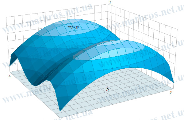
Then the surface \( z=f(x,y) \) lies above the \( xy \)-plane. The region \( D \) forms the base of a three-dimensional solid, while the value of the function determines its height at each point.
In this case,
\[
V=\iint_D f(x,y)\,dA
\]
gives the volume of the solid located above the region \( D \) and below the surface \( z=f(x,y) \).
The connection with the definite integral is easy to see here. For a function of one variable, the integral is related to the area between the graph and the \( x \)-axis. For a function of two variables, the double integral is related to a three-dimensional solid.
But what happens if \( f(x,y) \) takes negative values? In that case, the parts located below the \( xy \)-plane are counted with a minus sign. Therefore, in the general case, the value of a double integral should not be directly interpreted as an ordinary geometric volume.
Double Integral over a Rectangular Region: From a Double Integral to an Iterated Integral
Working directly with the limit of Riemann sums is not always convenient. In practice, a double integral is usually calculated using two definite integrals.
Consider the rectangular region
\[
D=\{(x,y)\mid a\leq x\leq b,\;c\leq y\leq d\}.
\]
If the function \( f(x,y) \) is continuous in this region, then the double integral can be written as an iterated integral:
\[
\iint_D f(x,y)\,dA
=
\int_a^b
\left(
\int_c^d f(x,y)\,dy
\right)dx.
\]
What happens in this expression? First, \( x \) is treated as a constant, and the function is integrated with respect to \( y \). After that, the resulting expression is integrated with respect to \( x \).
However, we can also proceed in the opposite order:
\[
\iint_D f(x,y)\,dA
=
\int_c^d
\left(
\int_a^b f(x,y)\,dx
\right)dy.
\]
Now \( y \) is treated as a constant, and the integration is first performed with respect to \( x \).
For a continuous function on a rectangular region, both orders lead to the same value:
\[
\int_a^b
\left(
\int_c^d f(x,y)\,dy
\right)dx
=
\int_c^d
\left(
\int_a^b f(x,y)\,dx
\right)dy.
\]
This result is connected with Fubini’s theorem. This theorem allows us to evaluate a double integral by calculating two definite integrals one after another.
Integration Region: How the Limits of Integration Are Defined
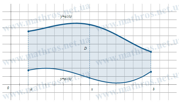
The region \( D \) does not have to be a rectangle. Its boundaries can be defined by functions, and in this case the limits of one of the integrals depend on the other variable.
If the region can be described by the conditions
\[
a\leq x\leq b,
\qquad
\varphi_1(x)\leq y\leq \varphi_2(x),
\]
then the double integral is written as
\[
\iint_D f(x,y)\,dA
=
\int_a^b
\left(
\int_{\varphi_1(x)}^{\varphi_2(x)}
f(x,y)\,dy
\right)dx.
\]
In this notation, for each fixed \( x \), the variable \( y \) ranges from the lower boundary \( \varphi_1(x) \) to the upper boundary \( \varphi_2(x) \). Geometrically, this means that the region can be viewed as a collection of vertical line segments between two boundary curves.
The region can also be described in the opposite way:
\[
c\leq y\leq d,
\qquad
\psi_1(y)\leq x\leq \psi_2(y).
\]
Then we have
\[
\iint_D f(x,y)\,dA
=
\int_c^d
\left(
\int_{\psi_1(y)}^{\psi_2(y)}
f(x,y)\,dx
\right)dy.
\]
Now, for each fixed \( y \), the variable \( x \) ranges from the left boundary \( \psi_1(y) \) to the right boundary \( \psi_2(y) \). In other words, we describe the same region using horizontal line segments.
Why is this important? The limits of an iterated integral directly describe the geometry of the region \( D \). Therefore, before calculating a double integral, we need to correctly determine the boundaries between which \( x \) and \( y \) vary.
In addition, the same region can often be described in both ways. In such a situation, the order of integration can be chosen depending on which form is more convenient.
Main Properties of Double Integrals: Rules for Working with Them
Double integrals have properties similar to those of a definite integral. This means that many familiar algebraic transformations can also be used here.
First of all, the linearity property holds. For constants \( \alpha \) and \( \beta \), we have
\[
\iint_D
\left(
\alpha\cdot f(x,y)+\beta\cdot g(x,y)
\right)\,dA
=
\alpha\cdot\iint_D f(x,y)\,dA
+
\beta\cdot\iint_D g(x,y)\,dA.
\]
Thus, a sum of functions can be integrated separately, while a constant factor can be taken outside the double integral.
Another important property is additivity with respect to the region of integration. If the region \( D \) consists of two parts \( D_1 \) and \( D_2 \) whose interiors do not overlap, then
\[
\iint_D f(x,y)\,dA
=
\iint_{D_1}f(x,y)\,dA
+
\iint_{D_2}f(x,y)\,dA.
\]
This means that a complex region can be divided into simpler parts, and each part can be considered separately.
The comparison property also holds. If, at every point of the region \( D \),
\[
f(x,y)\leq g(x,y),
\]
then
\[
\iint_D f(x,y)\,dA
\leq
\iint_D g(x,y)\,dA.
\]
In particular, if
\[
f(x,y)\geq 0
\]
throughout the region \( D \), then
\[
\iint_D f(x,y)\,dA\geq 0.
\]
Thus, a double integral preserves the main principles used with a definite integral. The main difference is that integration is now performed over a two-dimensional region, while the function depends on two variables.
Double Integral in Practice: Step-by-Step Calculation and Working with Limits
After looking at the definition and main properties, it is time to move on to actual calculations. Here, it is especially important to determine the region of integration correctly, write down the limits, and then calculate the inner and outer integrals step by step.
Example 1. Calculate the double integral
\[
\iint_D (x+2\cdot y)\,dA,
\]
if
\[
D=\{(x,y)\mid 0\leq x\leq 1,\;0\leq y\leq 2\}.
\]
The region \( D \) is a rectangle, so the limits of both integrals are constant. Let us write the double integral as an iterated integral:
\[
\iint_D (x+2\cdot y)\,dA
=
\int_0^1
\left(
\int_0^2
(x+2\cdot y)\,dy
\right)dx.
\]
First, we calculate the inner integral with respect to \( y \). Here, \( x \) is treated as a constant:
\[
\int_0^2
(x+2\cdot y)\,dy
=
\left.
\left(
x\cdot y+y^2
\right)
\right|_0^2.
\]
Substituting the limits, we get
\[
\left(
2\cdot x+4
\right)
–
0
=
2\cdot x+4.
\]
Now we only need to calculate the outer integral:
\[
\int_0^1
(2\cdot x+4)\,dx.
\]
We have
\[
\int_0^1
(2\cdot x+4)\,dx
=
\left.
\left(
x^2+4\cdot x
\right)
\right|_0^1.
\]
Therefore,
\[
1+4=5.
\]
So,
\[
\iint_D (x+2\cdot y)\,dA=5.
\]
Example 2. Calculate the double integral
\[
\iint_D x\cdot \cos(y)\,dA,
\]
if
\[
D=
\left\{
(x,y)
\mid
0\leq x\leq 2,\;
0\leq y\leq \frac{\pi}{2}
\right\}.
\]
Again, we have a rectangular region. Let us write the double integral as an iterated integral:
\[
\iint_D x\cdot \cos(y)\,dA
=
\int_0^2
\left(
\int_0^{\frac{\pi}{2}}
x\cdot \cos(y)\,dy
\right)dx.
\]
First, we integrate with respect to \( y \). Since \( x \) does not depend on \( y \), we can take it outside the inner integral:
\[
\int_0^{\frac{\pi}{2}}
x\cdot \cos(y)\,dy
=
x\cdot
\int_0^{\frac{\pi}{2}}
\cos(y)\,dy.
\]
We find the antiderivative:
\[
x\cdot
\left.
\sin(y)
\right|_0^{\frac{\pi}{2}}.
\]
Substituting the limits, we get
\[
x\cdot
\left(
\sin\left(\frac{\pi}{2}\right)-\sin(0)
\right)
=
x.
\]
Thus, the double integral reduces to
\[
\int_0^2 x\,dx.
\]
Now calculate:
\[
\int_0^2 x\,dx
=
\left.
\frac{x^2}{2}
\right|_0^2
=
\frac{4}{2}
=
2.
\]
Therefore,
\[
\iint_D x\cdot \cos(y)\,dA=2.
\]
Note. If the integrand can be written as a product of factors, each depending on only one variable, the calculation often becomes much simpler.
Example 3. Calculate the double integral
\[
\iint_D (x+y)\,dA,
\]
if the region \( D \) is defined by
\[
0\leq x\leq 1,
\qquad
0\leq y\leq 1-x.
\]
This time, the region of integration is not a rectangle. For each fixed \( x \), the variable \( y \) ranges from \( 0 \) to \( 1-x \).
Therefore, we write
\[
\iint_D (x+y)\,dA
=
\int_0^1
\left(
\int_0^{1-x}
(x+y)\,dy
\right)dx.
\]
First, we calculate the inner integral:
\[
\int_0^{1-x}
(x+y)\,dy
=
\left.
\left(
x\cdot y+\frac{y^2}{2}
\right)
\right|_0^{1-x}.
\]
After substituting the upper limit, we get
\[
x\cdot(1-x)
+
\frac{(1-x)^2}{2}.
\]
Expand the parentheses:
\[
x-x^2
+
\frac{1-2\cdot x+x^2}{2}.
\]
After simplifying, we obtain
\[
\frac{1}{2}
–
\frac{x^2}{2}.
\]
Therefore,
\[
\iint_D (x+y)\,dA
=
\int_0^1
\left(
\frac{1}{2}
–
\frac{x^2}{2}
\right)dx.
\]
We find the antiderivative:
\[
\left.
\left(
\frac{x}{2}
–
\frac{x^3}{6}
\right)
\right|_0^1.
\]
Substituting the limits, we get
\[
\frac{1}{2}
–
\frac{1}{6}
=
\frac{1}{3}.
\]
Therefore,
\[
\iint_D (x+y)\,dA
=
\frac{1}{3}.
\]
Here, the upper limit of the inner integral depends on \( x \). This dependence reflects the shape of the region \( D \).
Example 4. Calculate
\[
\iint_D 1\,dA,
\]
if the region \( D \) is defined by the conditions
\[
0\leq x\leq 2,
\qquad
x^2\leq y\leq 2\cdot x.
\]
For each \( x \) from \( 0 \) to \( 2 \), the variable \( y \) ranges from the curve
\[
y=x^2
\]
to the line
\[
y=2\cdot x.
\]
Therefore, the double integral has the form
\[
\iint_D 1\,dA
=
\int_0^2
\left(
\int_{x^2}^{2\cdot x}
1\,dy
\right)dx.
\]
We calculate the inner integral:
\[
\int_{x^2}^{2\cdot x}
1\,dy
=
\left.
y
\right|_{x^2}^{2\cdot x}.
\]
This gives
\[
2\cdot x-x^2.
\]
Now calculate the outer integral:
\[
\int_0^2
(2\cdot x-x^2)\,dx.
\]
We find the antiderivative:
\[
\left.
\left(
x^2-\frac{x^3}{3}
\right)
\right|_0^2.
\]
Substituting the limits, we get
\[
4-\frac{8}{3}
=
\frac{12}{3}-\frac{8}{3}
=
\frac{4}{3}.
\]
Therefore,
\[
\iint_D 1\,dA
=
\frac{4}{3}.
\]
Why is this case special? If the integrand is equal to \( 1 \), the value of the double integral is equal to the area of the region of integration.
Example 5. Calculate the double integral
\[
\iint_D 2\cdot x\,dA,
\]
if the region \( D \) is defined by
\[
0\leq y\leq 1,
\qquad
y\leq x\leq \sqrt{y}.
\]
In this case, the limits for \( y \) are given first, while the limits for \( x \) depend on \( y \). Therefore, it is convenient to integrate with respect to \( x \) first:
\[
\iint_D 2\cdot x\,dA
=
\int_0^1
\left(
\int_y^{\sqrt{y}}
2\cdot x\,dx
\right)dy.
\]
We calculate the inner integral:
\[
\int_y^{\sqrt{y}}
2\cdot x\,dx
=
\left.
x^2
\right|_y^{\sqrt{y}}.
\]
Substituting the limits, we get
\[
(\sqrt{y})^2-y^2.
\]
Since
\[
(\sqrt{y})^2=y,
\]
we obtain
\[
y-y^2.
\]
Now we have a definite integral:
\[
\int_0^1
(y-y^2)\,dy.
\]
We find the antiderivative:
\[
\left.
\left(
\frac{y^2}{2}
–
\frac{y^3}{3}
\right)
\right|_0^1.
\]
Substituting the limits, we get
\[
\frac{1}{2}
–
\frac{1}{3}
=
\frac{1}{6}.
\]
Therefore,
\[
\iint_D 2\cdot x\,dA
=
\frac{1}{6}.
\]
This example shows that \( x \) does not have to be the outer variable. The order of integration depends on how the region is defined and which form gives simpler limits.
From Double Integrals to Applications: What to Study Next
After learning about double integrals, you can continue exploring the practical applications of integral calculus. The following topics will show how integrals can be used to solve important geometric problems.
- Area of a Region Using an Integral: Formulas and Examples — We will look at how to use the definite integral to find the areas of regions bounded by graphs of functions.
- Volume of a Solid of Revolution: Applications of the Definite Integral — We will learn how the definite integral can be used to calculate the volumes of solids formed by rotating plane regions.
- Arc Length of a Curve: Formula Using the Definite Integral — We will explore how to use the definite integral to find the length of a part of a curve over a given interval.
Double Integral and Programming: Try to Implement the Algorithm Yourself
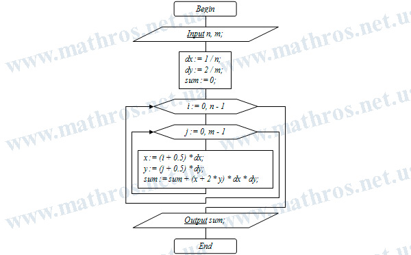
If you enjoy programming, try applying what you have learned about double integrals by creating your own program. The flowchart below shows an algorithm that approximately calculates the integral
\[
\iint_D (x+2\cdot y)\,dA,
\qquad
D=\{(x,y)\mid 0\leq x\leq1,\;0\leq y\leq2\}.
\]
The algorithm works by dividing the region into small rectangles. Follow the sequence of steps carefully, and then implement the algorithm in your favorite programming language. You can also try changing the number of subdivisions and observe how the calculated value approaches the exact result.