Romberg’s Method is one of the most effective techniques for numerical integration, combining the simplicity of the trapezoidal rule with the power of Richardson extrapolation. The main idea is to gradually increase the accuracy of calculations by reducing the integration step and refining the results using special formulas. This way, we achieve a much more precise result without performing unnecessary evaluations of the function.
Why Do We Need Romberg’s Method?
Let’s imagine we are calculating a definite integral using familiar methods like rectangles, trapezoids, or Simpson’s rule. All of them work by dividing the integration interval [a,b] into a certain number of parts. But do they always give us results that are accurate enough? Obviously, not always. The accuracy depends heavily on the choice of the step size h=(b-a)/n. If the function changes unevenly, the error can become quite large.
This is where Richardson extrapolation comes in to help. It allows us to make the result more accurate without adding extra function evaluations. In other words, we “squeeze out” the maximum benefit from the values we’ve already calculated.
How Romberg’s Method Works: Step by Step
So how does Romberg’s method actually work? We begin with the trapezoidal rule on the interval [a,b]. For the first approximation, we use just one interval. That gives us h0=b-a and the starting value:
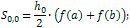
This is a rough estimate, but it’s the necessary starting point.
Next, we cut the step in half: h1=(b-a)/2. Instead of recalculating everything, we update the formula by adding only the new midpoint value of the function:

Now comes the first Richardson refinement. We combine S1,0 and S0,0 to eliminate the leading error of order h2:
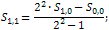
This gives us an improved approximation with second-order accuracy.
Moving to the third step, we halve the step again: h2=(b-a)/4. We add function values at new midpoints:

Then we refine along the first column:
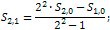
After this, we perform a second refinement, which removes error terms up to order h4:
At this stage, the accuracy is already much better than the trapezoidal rule with a moderate number of intervals.
The fourth step continues the same process. We take h3=(b-a)/8 and again add only the new midpoints:

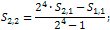
Then we refine along Romberg’s “diagonal“. First, the first column:
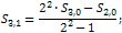
Next, the second column:
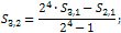
And finally, the third refinement increases the order by another two degrees:
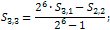
But when should we stop? A practical rule is to check the difference between successive refinements in the same row. If |Sk,j-Sk,j-1}|<ε, the desired accuracy has been reached. If not, we halve the step again, add new points, and continue.
This is how Romberg’s table is built: each row is more accurate than the previous one, and the final diagonal element Sk,k usually gives the best approximation of the integral.
Where to Start: Choosing the First Step
Do you always have to begin with h0=b-a? No. While this is the most common choice because it’s the simplest, it isn’t a strict requirement. You can also start with any value h0=(b-a)/m, for example with m=2 or m=4.
The important thing is to keep halving the step afterward so that the update structure and refinement formulas remain valid. In practice, it’s sometimes better to start with two or four subintervals if the function changes rapidly or if the very first trapezoidal step gives an approximation that’s too rough.
General Formulas of Romberg’s Method
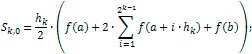
To complete the picture, let’s write down the general formulas. Suppose n=2k and hk=(b-a)/2k. Let Sk,0 be the approximation of the integral obtained by the composite trapezoidal rule on 2k subintervals. Then the basic formula is:
The efficient recursive update when halving the step is written as:

The Romberg refinements are then built using Richardson extrapolation:

This process creates the famous Romberg’s triangular table, where each diagonal element Sk,k is typically the most accurate approximation.
Accuracy and Error: What Exactly Are We Improving?
For the composite trapezoidal rule, there is a classical error estimate:

This means that if you halve the step size, the error decreases by about a factor of four.
But the real strength of Romberg’s method is that extrapolation increases the order of accuracy dramatically:

That’s why Romberg refinements Sk,k converge so quickly to the exact value.
At the same time, it’s important to remember that endlessly halving the step doesn’t make sense. Once the difference between refinements becomes comparable to rounding error, further improvements are no longer noticeable, and the calculations may even become unstable.
The practical rule is simple: stop when the condition |Sk,j-Sk,j-1|<ε is satisfied, where ε is the accuracy you’ve chosen for your problem.
Romberg’s Method in Practice: Step-by-Step Example
Now that we’ve explored the theory, it’s time to see Romberg’s method “in action”. Reading formulas is one thing, but watching how they work on a real example is much more convincing. Let’s go through a full problem from start to finish and see just how efficient and accurate this method really is.
Example 1: Calculating the Integral of f(x)=x2-5 on the Interval [-3, 3] with Accuracy ε=0.01

We start with step h0=(3-(-3))/2=3 and use the trapezoidal rule to get the initial value of the definite integral. To save time on manual calculations, we’ll take this starting value from an online calculator—quick and error-free.
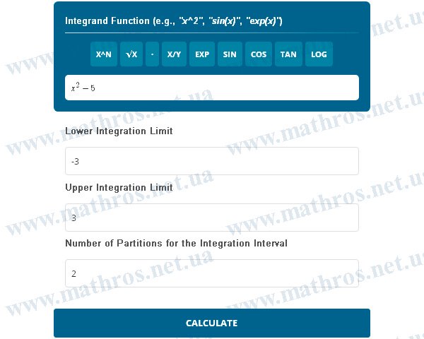
We enter the function, the integration limits, and the number of parts n=2. The calculator gives us the initial estimate.
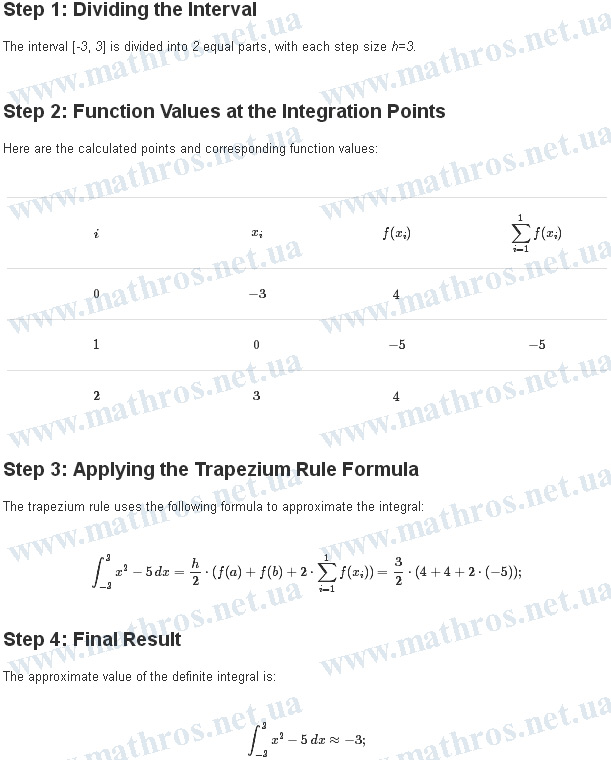
So, S0,0=-3. This is our starting base for Romberg’s method.
Next, we halve the step: h1=(3-(-3))/4=1.5. We update the trapezoidal sum by adding only the “new” midpoints a+(2⋅j-1)⋅h1 for j=1,2:

Now we refine the result with Richardson extrapolation:

To check stability, we halve again: h2=(3-(-3))/8=0.75. Adding new midpoints for j=1,2,3,4, we get:
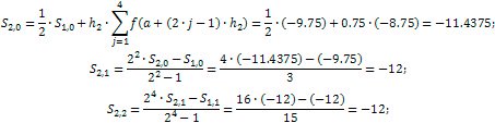
The stopping condition is satisfied here:

For completeness, let’s add one more row with h3=(3-(-3))/16=0.375 to confirm diagonal stability:
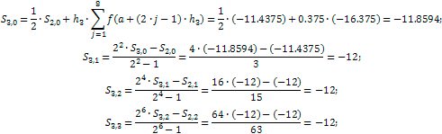
Romberg’s Table
| k/j | 0 | 1 | 2 | 3 |
|---|---|---|---|---|
| 0 | -3 | |||
| 1 | -9.75 | -12 | ||
| 2 | -11.4375 | -12 | -12 | |
| 3 | -11.8594 | -12 | -12 | -12 |
On the right side of the table, you can clearly see the rapid convergence to the exact value.
Let’s check analytically:

So, already at S2,2 we have convergence to machine precision. A great result with minimal extra calculations—exactly why Romberg’s method is so highly valued.
Where to Go Next: What to Study After Romberg’s Method
Do you want to deepen your understanding of integrals and see them in action beyond just the “area under a curve”? That’s a great idea. Here are three natural directions that build on what you’ve already learned. Pick one and move step by step, or explore all of them for an even fuller picture.
- Arc Length of a Curve: From Lines to Real Objects – Learn how definite integrals let you calculate the length of any curve, opening doors to geometry and physics applications.
- Area of a Plane Figure: When Curves Become Boundaries – Discover how integrals can be applied to find the area of shapes bounded by two curves, and use this knowledge for practical problems.
- Double Integrals with the Grid Method: A Step Toward Multidimensionality – Study the algorithm for computing double integrals over regions divided into cells, and understand how to integrate functions of two variables.
Ready to give it a try? Choose a topic and spend some time practicing – that way, your knowledge will solidify and start working for you in real-world problems.
Your Personal Tool: Romberg’s Method in Code
To wrap things up, let’s take one more step – bringing Romberg’s method into program code. Imagine how convenient it is when all the steps you once carried out by hand are now automated by your computer. This not only saves a huge amount of time but also guarantees high accuracy in your calculations.
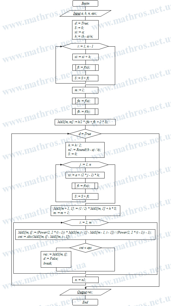
You can implement the algorithm in any programming language you prefer – from Python to C++ or Java. The flowchart shown below will serve as your guide: it clearly illustrates the sequence of actions and helps you transfer the mathematical method into code without any difficulties.
By doing this, you’ll create your own tool that delivers fast and reliable results, ready to handle even complex integration problems.