Rank of a matrix helps you understand how much useful, independent information a matrix contains, which is why it becomes a key characteristic in many linear algebra problems. In this article, we focus on the method of elementary transformations—an approach that lets you find the rank quickly, clearly, and without unnecessary calculations. You’ll see how this method works in practice, and you’ll learn how to confidently move from the original matrix to its echelon form, getting the rank without extra struggle.
Rank of a Matrix: Why Elementary Transformations Make Calculations Easier
Method of bordering minors reflects the definition of rank very well and gives an exact result. However, it requires computing a large number of determinants. For larger matrices, this quickly becomes time-consuming. That’s why, in practice, people often use the method of elementary transformations. The idea is simple: the rank of a matrix does not change if you apply certain allowed operations to it. So what operations are those?
Elementary transformations of a matrix include:
- Swapping any two rows or any two columns.
- Multiplying all elements of any chosen row or column by the same nonzero number.
- Adding to the elements of one row (or column) the corresponding elements of another row (or column), after first multiplying that other row (or column) by a nonzero number.
- Deleting rows or columns that consist only of zero elements.
The core idea of the method is this: using these transformations, the matrix \( A \) is reduced to echelon form. After that, only one final step remains—count the number of nonzero rows. That number is exactly the rank of the matrix. Convenient, right? On top of that, this approach is easy to implement in algorithms and software solutions.
Computation Algorithm: How to Reach an Echelon Matrix
Now let’s move to a more formal description. Suppose we have an \( m \times n \) matrix:
\[
A=\begin{pmatrix}
a_{11} & a_{12} & a_{13} & \dots & a_{1,n-2} & a_{1,n-1} & a_{1n}\\
a_{21} & a_{22} & a_{23} & \dots & a_{2,n-2} & a_{2,n-1} & a_{2n}\\
\vdots & \vdots & \vdots & \ddots & \vdots & \vdots & \vdots\\
a_{m1} & a_{m2} & a_{m3} & \dots & a_{m,n-2} & a_{m,n-1} & a_{mn}
\end{pmatrix}.
\]
Our goal is to use a sequence of elementary row transformations to obtain an echelon matrix.
So first, we eliminate all entries below the first diagonal element \( a_{11} \) in the first column. To do this, we replace rows \( 2,3,\dots,m \) in such a way that zeros appear under \( a_{11} \) (in other words, we “remove” the first-column entries below the pivot element). After this step, the matrix takes the form:
\[
A^{(1)}=\begin{pmatrix}
a_{11} & a_{12} & a_{13} & \dots & a_{1,n-2} & a_{1,n-1} & a_{1n}\\
0 & a^{(1)}_{22} & a^{(1)}_{23} & \dots & a^{(1)}_{2,n-2} & a^{(1)}_{2,n-1} & a^{(1)}_{2n}\\
\vdots & \vdots & \vdots & \ddots & \vdots & \vdots & \vdots\\
0 & a^{(1)}_{m2} & a^{(1)}_{m3} & \dots & a^{(1)}_{m,n-2} & a^{(1)}_{m,n-1} & a^{(1)}_{mn}
\end{pmatrix},
\]
where the entries with the superscript \( (1) \) are computed by:
\[
a_{ij}^{(1)} = a_{ij} – \frac{a_{i1}}{a_{11}} \cdot a_{1j}; \quad i=2,\dots,m; \quad j=1,\dots,n.
\]
Next, we exclude the first row and the first column and apply the same idea to the submatrix that starts at the element \( a^{(1)}_{22} \). Now we need to eliminate all entries below \( a^{(1)}_{22} \) in the second column. After that, we get:
\[
A^{(2)}=\begin{pmatrix}
a_{11} & a_{12} & a_{13} & \dots & a_{1,{n-2}} & a_{1,{n-1}} & a_{1n}\\
0 & a^{(1)}_{22} & a^{(1)}_{23} & \dots & a^{(1)}_{2,{n-2}} & a^{(1)}_{2,{n-1}} & a^{(1)}_{2n}\\
0 & 0 & a^{(2)}_{33} & \dots & a^{(2)}_{3,{n-2}} & a^{(2)}_{3,{n-1}} & a^{(2)}_{3n}\\
\vdots & \vdots & \vdots & \ddots & \vdots & \vdots & \vdots\\
0 & 0 & a^{(2)}_{m3} & \dots & a^{(2)}_{m,{n-2}} & a^{(2)}_{m,{n-1}} & a^{(2)}_{mn}
\end{pmatrix},
\]
where
\[
a_{ij}^{(2)} = a_{ij}^{(1)} – \frac{a_{i2}^{(1)}}{a_{22}^{(1)}} \cdot a_{2j}^{(1)}; \quad i=3,\dots,m; \quad j=2,\dots,n.
\]
By continuing this process for each next column, at the \( (m-1) \)-th step the matrix reaches an echelon (triangular) form:
\[
A^{(m-1)}=\begin{pmatrix}
a_{11} & a_{12} & a_{13} & \dots & a_{1,n-2} & a_{1,n-1} & a_{1n}\\
0 & a^{(1)}_{22} & a^{(1)}_{23} & \dots & a^{(1)}_{2,n-2} & a^{(1)}_{2,n-1} & a^{(1)}_{2n}\\
0 & 0 & a^{(2)}_{33} & \dots & a^{(2)}_{3,n-2} & a^{(2)}_{3,n-1} & a^{(2)}_{3n}\\
\vdots & \vdots & \vdots & \ddots & \vdots & \vdots & \vdots\\
0 & 0 & 0 & \dots & a^{(m-1)}_{m,n-2} & a^{(m-1)}_{m,n-1} & a^{(m-1)}_{mn}
\end{pmatrix}.
\]
A general formula for the entries at step \( k \) looks like this:
\[
a_{ij}^{(k)} = a_{ij}^{(k-1)} – \frac{a_{ik}^{(k-1)}}{a_{kk}^{(k-1)}} \cdot a_{kj}^{(k-1)};
\quad k = 1,\dots,m-1; \quad i = k+1,\dots,m; \quad j = k,\dots,n.
\]
Once the matrix is in echelon form, we count how many nonzero rows it has. That number is exactly the rank of the matrix.
Note. In practice, it can happen that the pivot element you want to start with (for example \( a_{11} \), or later \( a^{(1)}_{22} \), \( a^{(2)}_{33} \), and so on) is equal to zero. In that case, it’s enough to swap rows (or, if needed, columns) so that a nonzero number appears in the pivot position. Since swapping is an elementary transformation, the rank does not change, and you can continue the elimination process as usual. If, in the same column, all entries below are also zero, then this column does not provide a new pivot element, and you move on to the next column.
Practical Part: Rank of a Matrix Using Elementary Transformations in Examples
Theory gives you the big picture, but real confidence shows up when you personally reduce a matrix to echelon form and clearly see the result. So below we’ll work through three typical problems and track, step by step, how elementary transformations lead to the rank value. In every example, the final conclusion is the same: the rank equals the number of nonzero rows in the echelon form.
Example 1: Find the rank of a 3×3 matrix
\[
A=\begin{pmatrix}
1 & 0 & 2\\
0 & 1 & 3\\
4 & 5 & 6
\end{pmatrix}.
\]
We start with the first column. Our goal is to make all entries below \( a_{11}=1 \) equal to zero. Since the second row already has a zero in the first column, we leave that row unchanged. For the third row, we add the first row multiplied by \( -\frac{a_{31}}{a_{11}}=-\frac{4}{1}=-4 \). After this transformation, we get:
\[
A^{(1)}=\begin{pmatrix}
1 & 0 & 2\\
0 & 1 & 3\\
0 & 5 & -2
\end{pmatrix}.
\]
Now we work with the second column and aim to eliminate the entry below the diagonal element \( a^{(1)}_{22}=1 \). So we add the second row multiplied by \( -\frac{a^{(1)}_{32}}{a^{(1)}_{22}}=-\frac{5}{1}=-5 \) to the third row. As a result, we obtain:
\[
A^{(2)}=\begin{pmatrix}
1 & 0 & 2\\
0 & 1 & 3\\
0 & 0 & -17
\end{pmatrix}.
\]
The matrix is now in echelon form, and all three rows are nonzero. Therefore, \( \mathrm{rank}A=3 \).
Example 2: Find the rank of a 3×3 matrix
\[
A=\begin{pmatrix}
2 & -1 & 4\\
4 & -2 & 8\\
6 & -3 & 12
\end{pmatrix}.
\]
We begin with the first column and eliminate the entries below \( a_{11}=2 \). We add the first row multiplied by \( -\frac{a_{21}}{a_{11}}=-\frac{4}{2}=-2 \) to the second row, and we add the first row multiplied by \( -\frac{a_{31}}{a_{11}}=-\frac{6}{2}=-3 \) to the third row. After that, we have:
\[
A^{(1)}=\begin{pmatrix}
2 & -1 & 4\\
0 & 0 & 0\\
0 & 0 & 0
\end{pmatrix}.
\]
The matrix is essentially already in echelon form: only the first row remains nonzero, while the other two have become zero rows. So the number of nonzero rows is \( 1 \), which means \( \mathrm{rank}A=1 \).
Example 3: Find the rank of a 4×5 matrix
\[
A=\begin{pmatrix}
0 & -1 & 3 & 0 & 2\\
2 & -4 & 1 & 5 & 3\\
-4 & 5 & 7 & -10 & 0\\
-2 & 1 & 8 & -5 & 3
\end{pmatrix}.
\]
In the first column, the first row starts with a zero, so it’s convenient to swap the first and second rows to get a nonzero pivot element. After swapping, we get:
\[
A=\begin{pmatrix}
2 & -4 & 1 & 5 & 3\\
0 & -1 & 3 & 0 & 2\\
-4 & 5 & 7 & -10 & 0\\
-2 & 1 & 8 & -5 & 3
\end{pmatrix}.
\]
Now we eliminate the entries below \( a_{11}=2 \). To the third row, we add the first row multiplied by \( -\frac{a_{31}}{a_{11}}=-\left(\frac{-4}{2}\right)=2 \). To the fourth row, we add the first row multiplied by \( -\frac{a_{41}}{a_{11}}=-\left(\frac{-2}{2}\right)=1 \). This gives:
\[
A^{(1)}=\begin{pmatrix}
2 & -4 & 1 & 5 & 3\\
0 & -1 & 3 & 0 & 2\\
0 & -3 & 9 & 0 & 6\\
0 & -3 & 9 & 0 & 6
\end{pmatrix}.
\]
Next we move to the second column. The pivot element here is \( a^{(1)}_{22}=-1 \). We eliminate the entries below it: to the third row we add the second row multiplied by \( -\frac{a^{(1)}_{32}}{a^{(1)}_{22}}=-\frac{-3}{-1}=-3 \), and we do the same for the fourth row (also multiply the second row by \( -3 \) and add it). We obtain:
\[
A^{(2)}=\begin{pmatrix}
2 & -4 & 1 & 5 & 3\\
0 & -1 & 3 & 0 & 2\\
0 & 0 & 0 & 0 & 0\\
0 & 0 & 0 & 0 & 0
\end{pmatrix}.
\]
The matrix is now in echelon form, and exactly two rows remain nonzero. Therefore, \( \mathrm{rank}A=2 \).
Where to Go After Rank: What Topics Best Continue Your Practice?
If you enjoyed using elementary transformations to compute rank, you probably don’t want to stop here, right? The best next step is to move on to topics where the very same transformations unlock even more useful ideas in matrices and systems of equations.
- Inverse Matrix: How Elementary Transformations Lead to the Result — We’ll break down how these transformations help you find an inverse matrix.
- Determinant of a Matrix: Elementary Transformations as a Path to Triangular Form — You’ll learn how to reduce a matrix to triangular form and compute the determinant.
- Systems of Equations: Gaussian Elimination as the Main Solving Tool — We’ll explain how row transformations produce solutions for systems.
From a Flowchart to Code: Rank of a Matrix in Your Program
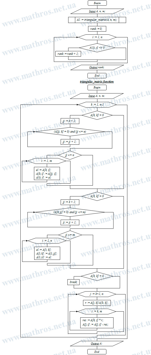
If you’re interested in programming, a flowchart of the algorithm for computing a matrix rank using elementary transformations can be a great starting point for a small program in your favorite language. Take a close look at the diagram, follow the path from the input matrix to the final result, and imagine how each block can turn into a clear piece of code. Isn’t it tempting to implement this in Python, C++, Java, or any other language, so you can get the rank of matrices of different sizes with a single run? This kind of exercise helps you reinforce the topic and, at the same time, trains the skill of translating a ready-made flowchart logic into a working program.