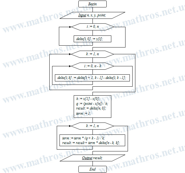
Newton’s backward interpolation formula makes it possible to approximate function values from tabulated data at equally spaced nodes. It is usually applied when the interpolation point is located near the end of the table. Let us explore how to construct the interpolation polynomial, transform it into a convenient computational form, and apply it when solving examples step by step.
Construction from the Last Node: The Polynomial and Generalized Power
Suppose that the values
\[
y_i=f(x_i), \qquad i=0,1,2,\dots,n,
\]
are known for the function \( y=f(x) \) at the interpolation nodes
\[
x_i=x_0+i\cdot h,
\]
where the nodes are arranged in ascending order and \( h>0 \) is the constant step between neighboring nodes.
For \( n+1 \) distinct nodes, there is a unique polynomial \( P_n(x) \) whose degree does not exceed \( n \) and which satisfies the interpolation conditions
\[
P_n(x_i)=y_i, \qquad i=0,1,2,\dots,n.
\]
At the interpolation nodes, the polynomial values exactly match the given function values. At other points, the polynomial is used to approximate the function values.
The construction of Newton’s backward formula begins at the last node \( x_n \). Therefore, we will look for the interpolation polynomial in the form
\[
P_n(x)=a_0+a_1\cdot(x-x_n)+a_2\cdot(x-x_n)\cdot(x-x_{n-1})+\dots+a_n\cdot(x-x_n)\cdot(x-x_{n-1})\cdot\dots\cdot(x-x_1),
\]
where \( a_0,a_1,\dots,a_n \) are unknown coefficients.
Each successive term contains one additional factor associated with the preceding node in the table. To make this notation shorter, let us introduce the generalized power:
\[
\begin{gathered}
(x-x_n)^{[0]}=1,\\[4pt]
(x-x_n)^{[k]}=(x-x_n)\cdot(x-x_{n-1})\cdot\dots\cdot(x-x_{n-k+1}), \qquad k\geq1.
\end{gathered}
\]
In Newton’s backward formula, the generalized power is formed starting from the last node and continuing toward nodes with smaller indices. For example,
\[
\begin{gathered}
(x-x_n)^{[1]}=x-x_n,\\[4pt]
(x-x_n)^{[2]}=(x-x_n)\cdot(x-x_{n-1}),\\[4pt]
(x-x_n)^{[3]}=(x-x_n)\cdot(x-x_{n-1})\cdot(x-x_{n-2}).
\end{gathered}
\]
Using this notation, the interpolation polynomial can be written more compactly:
\[
P_n(x)=a_0+a_1\cdot(x-x_n)^{[1]}+a_2\cdot(x-x_n)^{[2]}+\dots+a_n\cdot(x-x_n)^{[n]}.
\]
The generalized power should not be confused with the ordinary power. For example,
\[
(x-x_n)^{[2]}=(x-x_n)\cdot(x-x_{n-1}),
\]
whereas
\[
(x-x_n)^2=(x-x_n)\cdot(x-x_n).
\]
In the first case, the product contains factors associated with different interpolation nodes. In the second case, the same factor is repeated twice. Therefore, these expressions have different structures and, in general, different values.
Backward Finite Differences: Forming the Lower Diagonal of the Table
Since the polynomial construction begins at the last node, it is convenient to express its coefficients using backward finite differences.
For an arbitrary function \( g(x) \), the first-order backward finite difference is defined as
\[
\nabla g(x)=g(x)-g(x-h).
\]
If \( x=x_i \), then
\[
x_i-h=x_{i-1}.
\]
Therefore, the backward finite difference shows how the function value changes when moving from the previous node to the current one.
For tabulated function values, the first-order difference has the form
\[
\nabla y_i=y_i-y_{i-1}.
\]
In particular,
\[
\begin{gathered}
\nabla y_n=y_n-y_{n-1},\\[4pt]
\nabla y_{n-1}=y_{n-1}-y_{n-2}.
\end{gathered}
\]
The second-order backward difference is calculated using first-order differences:
\[
\nabla^2y_i=\nabla y_i-\nabla y_{i-1}.
\]
For example,
\[
\nabla^2y_n=\nabla y_n-\nabla y_{n-1}.
\]
In general, the \( k \)-th-order backward finite difference is defined recursively:
\[
\nabla^ky_i=\nabla^{k-1}y_i-\nabla^{k-1}y_{i-1}.
\]
Differences of each successive order are calculated from two neighboring differences of the previous order. For \( n+1 \) tabulated values, finite differences up to and including the \( n \)-th order can be calculated.
Newton’s backward formula uses the last function value and backward differences of all orders calculated at the last node:
\[
y_n,\qquad \nabla y_n,\qquad \nabla^2y_n,\qquad \dots,\qquad \nabla^ny_n.
\]
Backward differences are related to forward finite differences. For the first order, we have
\[
\nabla y_n=y_n-y_{n-1}=\Delta y_{n-1}.
\]
For the second order, the following equality holds:
\[
\nabla^2y_n=\Delta^2y_{n-2}.
\]
In general,
\[
\nabla^ky_n=\Delta^ky_{n-k}.
\]
Therefore, it is not necessary to construct a separate table of backward differences. Instead, we can create a standard table of forward finite differences and select the following values from it:
\[
\Delta y_{n-1},\qquad \Delta^2y_{n-2},\qquad \Delta^3y_{n-3},\qquad \dots,\qquad \Delta^ny_0.
\]
These elements form the lower diagonal of the difference table and correspond to the backward differences calculated at the last node.
Newton’s Backward Interpolation Formula: Sequential Determination of the Coefficients
First, let us find the coefficient \( a_0 \). To do this, substitute \( x=x_n \) into the polynomial. All terms except the first contain the factor \( x-x_n \), so they become zero:
\[
P_n(x_n)=a_0.
\]
According to the interpolation condition,
\[
P_n(x_n)=y_n.
\]
Therefore,
\[
a_0=y_n.
\]
To find the remaining coefficients, apply the backward finite-difference operator to the polynomial:
\[
\nabla P_n(x)=P_n(x)-P_n(x-h).
\]
For the generalized power introduced earlier, the following relation holds:
\[
\nabla(x-x_n)^{[k]}=k\cdot h\cdot(x-x_n)^{[k-1]}.
\]
Each application of the backward-difference operator reduces the order of the generalized power by one and introduces the corresponding numerical factor and a factor of \( h \).
After calculating the first backward difference and substituting \( x=x_n \), we obtain
\[
\nabla P_n(x_n)=a_1\cdot h.
\]
On the other hand,
\[
\nabla P_n(x_n)=P_n(x_n)-P_n(x_n-h).
\]
Since
\[
x_{n-1}=x_n-h,
\]
we have
\[
\nabla P_n(x_n)=P_n(x_n)-P_n(x_{n-1}).
\]
At the interpolation nodes, the polynomial values match the tabulated function values. Therefore,
\[
\nabla P_n(x_n)=y_n-y_{n-1}=\nabla y_n.
\]
It follows that
\[
a_1=\frac{\nabla y_n}{h}.
\]
To determine the coefficient \( a_2 \), calculate the second-order backward finite difference. After substituting \( x=x_n \), we obtain
\[
\nabla^2P_n(x_n)=2!\cdot a_2\cdot h^2.
\]
Since
\[
\nabla^2P_n(x_n)=\nabla^2y_n,
\]
we get
\[
a_2=\frac{\nabla^2y_n}{2!\cdot h^2}.
\]
Continuing this process, for the \( k \)-th-order difference we obtain
\[
\nabla^kP_n(x_n)=k!\cdot a_k\cdot h^k.
\]
Therefore,
\[
a_k=\frac{\nabla^ky_n}{k!\cdot h^k}, \qquad k=1,2,\dots,n.
\]
Substituting the coefficients into the polynomial gives
\[
P_n(x)=y_n+\frac{\nabla y_n}{1!\cdot h}\cdot(x-x_n)^{[1]}+\frac{\nabla^2y_n}{2!\cdot h^2}\cdot(x-x_n)^{[2]}+\dots+\frac{\nabla^ny_n}{n!\cdot h^n}\cdot(x-x_n)^{[n]}.
\]
Using the relationship between backward and forward differences, this polynomial can also be written as
\[
P_n(x)=y_n+\frac{\Delta y_{n-1}}{1!\cdot h}\cdot(x-x_n)^{[1]}+\frac{\Delta^2y_{n-2}}{2!\cdot h^2}\cdot(x-x_n)^{[2]}+\dots+\frac{\Delta^ny_0}{n!\cdot h^n}\cdot(x-x_n)^{[n]}.
\]
The resulting expression is an intermediate form of the interpolation polynomial written using generalized powers. For direct calculations, we will now rewrite it using a normalized variable.
Normalized Variable: Converting the Formula into a Practical Form
Let us introduce the variable
\[
q=\frac{x-x_n}{h}.
\]
It shows the displacement of the point \( x \) from the last node \( x_n \), measured in units of the step \( h \). Therefore,
\[
x-x_n=q\cdot h.
\]
Since
\[
x_{n-j}=x_n-j\cdot h,
\]
we have
\[
x-x_{n-j}=x-x_n+j\cdot h=q\cdot h+j\cdot h=(q+j)\cdot h.
\]
Thus,
\[
\begin{gathered}
x-x_{n-1}=(q+1)\cdot h,\\[4pt]
x-x_{n-2}=(q+2)\cdot h,
\end{gathered}
\]
and, in general,
\[
x-x_{n-j}=(q+j)\cdot h.
\]
Therefore, the generalized power can be written as
\[
(x-x_n)^{[k]}=h^k\cdot q\cdot(q+1)\cdot(q+2)\cdot\dots\cdot(q+k-1).
\]
Let us examine this transformation for the second-order term:
\[
\frac{\nabla^2y_n}{2!\cdot h^2}\cdot h^2\cdot q\cdot(q+1)=\frac{q\cdot(q+1)}{2!}\cdot\nabla^2y_n.
\]
The factor \( h^2 \) that appears in the generalized power cancels with the same factor in the denominator of the coefficient. A similar cancellation occurs in every subsequent term.
As a result, we obtain Newton’s Backward Interpolation Formula:
\[
P_n(x)=y_n+q\cdot\nabla y_n+\frac{q\cdot(q+1)}{2!}\cdot\nabla^2y_n+\frac{q\cdot(q+1)\cdot(q+2)}{3!}\cdot\nabla^3y_n+\dots+\frac{q\cdot(q+1)\cdot(q+2)\cdot\dots\cdot(q+n-1)}{n!}\cdot\nabla^ny_n.
\]
Using forward finite differences, this formula takes the form
\[
\begin{gathered}
P_n(x)=y_n+q\cdot\Delta y_{n-1}
+\frac{q\cdot(q+1)}{2!}\cdot\Delta^2 y_{n-2}
+\frac{q\cdot(q+1)\cdot(q+2)}{3!}\cdot\Delta^3 y_{n-3}+\cdots\\[4pt]
+\frac{q\cdot(q+1)\cdot(q+2)\cdot\cdots\cdot(q+n-1)}{n!}\cdot\Delta^n y_0.
\end{gathered}
\]
If the point \( x \) lies between the last two nodes \( x_{n-1} \) and \( x_n \), then
\[
-1\leq q\leq0.
\]
For example, \( q=-0.5 \) means that the point \( x \) lies half a step to the left of \( x_n \).
Newton’s backward interpolation formula is usually applied when the point \( x \) is located near the last node \( x_n \). In this case, the value of \( |q| \) is small, and the factors in the formula are convenient for calculations.
If all differences up to the \( n \)-th order are included, Newton’s forward and backward formulas are simply different forms of the same interpolation polynomial. The difference lies in the node from which the construction begins and in the order in which the tabulated differences are used. For this reason, Newton’s backward interpolation formula is also called Newton’s backward formula.
Newton’s Backward Interpolation Formula: Step-by-Step Examples
Let us apply the formula to tables with different numbers of equally spaced nodes. We will calculate the finite differences, determine the normalized variable, and find approximate function values step by step.
Example 1. Using the tabulated function values below, find an approximate value of \( f(2.5) \)
| \( i \) | \( x_i \) | \( y_i \) |
|---|---|---|
| \( 0 \) | \( 1 \) | \( 1 \) |
| \( 1 \) | \( 2 \) | \( 4 \) |
| \( 2 \) | \( 3 \) | \( 9 \) |
The nodes are equally spaced. The interpolation step is
\[
h=x_1-x_0=2-1=1.
\]
Let us calculate the first-order finite differences:
\[
\Delta y_0=y_1-y_0=4-1=3,
\qquad
\Delta y_1=y_2-y_1=9-4=5.
\]
Now find the second-order finite difference:
\[
\Delta^2y_0=\Delta y_1-\Delta y_0=5-3=2.
\]
The calculated values can be arranged in a finite-difference table.
| \( i \) | \( x_i \) | \( y_i \) | \( \Delta y_i \) | \( \Delta^2y_i \) |
|---|---|---|---|---|
| \( 0 \) | \( 1 \) | \( 1 \) | \( 3 \) | \( 2 \) |
| \( 1 \) | \( 2 \) | \( 4 \) | \( 5 \) | — |
| \( 2 \) | \( 3 \) | \( 9 \) | — | — |
Let us calculate the normalized variable relative to the last node \( x_2=3 \):
\[
q=\frac{x-x_2}{h}=\frac{2.5-3}{1}=-0.5.
\]
For three nodes, Newton’s Backward Interpolation Formula takes the form
\[
P_2(x)=y_2+q\cdot\Delta y_1+\frac{q\cdot(q+1)}{2!}\cdot\Delta^2y_0.
\]
From the lower diagonal of the table, we take the values
\[
y_2=9,
\qquad
\Delta y_1=5,
\qquad
\Delta^2y_0=2.
\]
We substitute the following values into the formula:
\[
P_2(2.5)=9-0.5\cdot5+\frac{(-0.5)\cdot(-0.5+1)}{2!}\cdot2.
\]
Now perform the calculations:
\[
P_2(2.5)=9-2.5-0.25=6.25.
\]
Therefore,
\[
f(2.5)\approx6.25.
\]
Example 2. Using the tabulated function values below, find an approximate value of \( f(2.3) \)
| \( i \) | \( x_i \) | \( y_i \) |
|---|---|---|
| \( 0 \) | \( 1 \) | \( 5 \) |
| \( 1 \) | \( 1.5 \) | \( 8.375 \) |
| \( 2 \) | \( 2 \) | \( 4 \) |
| \( 3 \) | \( 2.5 \) | \( 22.625 \) |
The step between neighboring nodes is
\[
h=x_1-x_0=1.5-1=0.5.
\]
Let us calculate the finite differences up to the third order:
\[
\begin{gathered}
\Delta y_0=8.375-5=3.375,
\qquad
\Delta y_1=14-8.375=5.625,
\qquad
\Delta y_2=22.625-14=8.625,\\[4pt]
\Delta^2y_0=5.625-3.375=2.25,
\qquad
\Delta^2y_1=8.625-5.625=3,\\[4pt]
\Delta^3y_0=3-2.25=0.75.
\end{gathered}
\]
The results can be arranged in the following table.
| \( i \) | \( x_i \) | \( y_i \) | \( \Delta y_i \) | \( \Delta^2y_i \) | \( \Delta^3y_i \) |
|---|---|---|---|---|---|
| \( 0 \) | \( 1 \) | \( 5 \) | \( 3.375 \) | \( 2.25 \) | \( 0.75 \) |
| \( 1 \) | \( 1.5 \) | \( 8.375 \) | \( 5.625 \) | \( 3 \) | — |
| \( 2 \) | \( 2 \) | \( 14 \) | \( 8.625 \) | — | — |
| \( 3 \) | \( 2.5 \) | \( 22.625 \) | — | — | — |
The last node is \( x_3=2.5 \). Let us calculate \( q \):
\[
q=\frac{x-x_3}{h}=\frac{2.3-2.5}{0.5}=-0.4.
\]
For four nodes, we use the formula
\[
P_3(x)=y_3+q\cdot\Delta y_2+\frac{q\cdot(q+1)}{2!}\cdot\Delta^2y_1+\frac{q\cdot(q+1)\cdot(q+2)}{3!}\cdot\Delta^3y_0.
\]
We substitute the following values into the formula:
\[
y_3=22.625,
\qquad
\Delta y_2=8.625,
\qquad
\Delta^2y_1=3,
\qquad
\Delta^3y_0=0.75.
\]
Substituting the calculated values gives
\[
P_3(2.3)=22.625-0.4\cdot8.625+\frac{(-0.4)\cdot(-0.4+1)}{2!}\cdot3+\frac{(-0.4)\cdot(-0.4+1)\cdot(-0.4+2)}{3!}\cdot0.75.
\]
Now calculate the individual terms:
\[
\begin{gathered}
-0.4\cdot8.625=-3.45,\\[4pt]
\frac{(-0.4)\cdot0.6}{2!}\cdot3=-0.36,\\[4pt]
\frac{(-0.4)\cdot0.6\cdot1.6}{3!}\cdot0.75=-0.048.
\end{gathered}
\]
Therefore,
\[
P_3(2.3)=22.625-3.45-0.36-0.048=18.767.
\]
Thus,
\[
f(2.3)\approx18.767.
\]
Example 3. Using the tabulated function values below, find an approximate value of \( f(7.2) \)
| \( i \) | \( x_i \) | \( y_i \) |
|---|---|---|
| \( 0 \) | \( 0 \) | \( 2 \) |
| \( 1 \) | \( 2 \) | \( 2 \) |
| \( 2 \) | \( 4 \) | \( 12 \) |
| \( 3 \) | \( 6 \) | \( 68 \) |
| \( 4 \) | \( 8 \) | \( 230 \) |
The interpolation step is
\[
h=x_1-x_0=2-0=2.
\]
Using the tabulated values, let us calculate the finite differences up to the fourth order:
\[
\begin{gathered}
\Delta y_0=2-2=0,
\qquad
\Delta y_1=12-2=10,
\qquad
\Delta y_2=68-12=56,
\qquad
\Delta y_3=230-68=162,\\[4pt]
\Delta^2y_0=10-0=10,
\qquad
\Delta^2y_1=56-10=46,
\qquad
\Delta^2y_2=162-56=106,\\[4pt]
\Delta^3y_0=46-10=36,
\qquad
\Delta^3y_1=106-46=60,\\[4pt]
\Delta^4y_0=60-36=24.
\end{gathered}
\]
The calculated results can be arranged in the following table.
| \( i \) | \( x_i \) | \( y_i \) | \( \Delta y_i \) | \( \Delta^2y_i \) | \( \Delta^3y_i \) | \( \Delta^4y_i \) |
|---|---|---|---|---|---|---|
| \( 0 \) | \( 0 \) | \( 2 \) | \( 0 \) | \( 10 \) | \( 36 \) | \( 24 \) |
| \( 1 \) | \( 2 \) | \( 2 \) | \( 10 \) | \( 46 \) | \( 60 \) | — |
| \( 2 \) | \( 4 \) | \( 12 \) | \( 56 \) | \( 106 \) | — | — |
| \( 3 \) | \( 6 \) | \( 68 \) | \( 162 \) | — | — | — |
| \( 4 \) | \( 8 \) | \( 230 \) | — | — | — | — |
The last node is \( x_4=8 \). Let us find the value of \( q \):
\[
q=\frac{x-x_4}{h}=\frac{7.2-8}{2}=-0.4.
\]
For five nodes, Newton’s Backward Interpolation Formula takes the form
\[
P_4(x)=y_4+q\cdot\Delta y_3+\frac{q\cdot(q+1)}{2!}\cdot\Delta^2y_2+\frac{q\cdot(q+1)\cdot(q+2)}{3!}\cdot\Delta^3y_1+\frac{q\cdot(q+1)\cdot(q+2)\cdot(q+3)}{4!}\cdot\Delta^4y_0.
\]
We substitute the following values into the formula:
\[
y_4=230,
\qquad
\Delta y_3=162,
\qquad
\Delta^2y_2=106,
\qquad
\Delta^3y_1=60,
\qquad
\Delta^4y_0=24.
\]
Substituting the calculated values gives
\[
\begin{gathered}
P_4(7.2)=230-0.4\cdot162+\frac{(-0.4)\cdot(-0.4+1)}{2!}\cdot106+\frac{(-0.4)\cdot(-0.4+1)\cdot(-0.4+2)}{3!}\cdot60+\\[4pt]
+\frac{(-0.4)\cdot(-0.4+1)\cdot(-0.4+2)\cdot(-0.4+3)}{4!}\cdot24.
\end{gathered}
\]
Now calculate the individual terms:
\[
\begin{gathered}
-0.4\cdot162=-64.8,\\[4pt]
\frac{(-0.4)\cdot0.6}{2!}\cdot106=-12.72,\\[4pt]
\frac{(-0.4)\cdot0.6\cdot1.6}{3!}\cdot60=-3.84,\\[4pt]
\frac{(-0.4)\cdot0.6\cdot1.6\cdot2.6}{4!}\cdot24\approx-0.998.
\end{gathered}
\]
Therefore,
\[
P_4(7.2)\approx230-64.8-12.72-3.84-0.998=147.642.
\]
Thus,
\[
f(7.2)\approx147.642.
\]
What to Study Next: Topics for Further Learning
You already know how to construct Newton’s polynomial from the end of a table and find approximate function values. Now it is worth exploring other methods for working with tabulated data and comparing their capabilities.
- Lagrange Interpolation Formula: Calculations for Unequally Spaced Nodes — This article will explain how to construct the Lagrange polynomial for unequally spaced nodes and calculate a function value step by step.
- Least Squares Method: Approximating Functions from Data — You will learn how to choose a function that best describes a data set by minimizing the differences between the tabulated and approximate values.
- Linear Interpolation: Approximating a Tabulated Function — We will examine a simple method for finding intermediate values from two neighboring nodes and determine when it gives an exact result.
Newton’s Backward Interpolation Formula: From Flowchart to Code
Do you enjoy programming? Then try implementing the algorithm shown in the flowchart using your favorite programming language. The program should create a finite-difference table, calculate the normalized variable relative to the last node, and find an approximate function value. Pascal, Python, JavaScript, or C++—the choice is yours. This will help you deepen your understanding of Newton’s Backward Interpolation Formula and see how a sequence of mathematical calculations can be turned into code.