Jacobi Method Explained: Your Step-by-Step Guide

Have you ever wondered how to find approximate solutions to a system of linear equations when direct methods become too complicated? The answer is simple – the Jacobi method! In this article, we’ll dive into how this iterative method works, the conditions necessary for its convergence, and how to apply it step by step. Together, we’ll explore examples, the matrix form of the method, and examine when this approach is truly effective. Ready to learn more about the Jacobi method? Let’s get started!

Jacobi Method: The Core Idea and How It Works

The Jacobi method is a numerical approach that allows you to find approximate solutions to systems of linear equations, step by step. Its main idea? Start with any initial values for the unknowns and gradually refine them. But how exactly does this work? At each step, we compute new values for each variable using the current values of the other variables. The iterations continue until the difference between consecutive results becomes so small that the solution can be considered accurate. It’s a simple and effective method, especially for systems with many equations.

How Does the Jacobi Method Algorithm Work?

Let’s take a closer look at how to implement the Jacobi method in practice. Imagine a system with n equations and n unknowns:

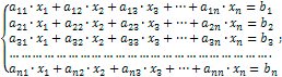
To use the Jacobi method, we assume that the diagonal coefficients a_ii≠0 for all i=1,…,n. We can then rewrite each equation in the system so that each variable can be calculated separately. For example, we solve the first equation for x₁, the second for x₂, the third for x₃ and so on.

The result is a new system of equations that looks like this:

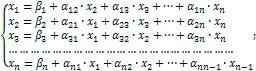
Here, β_i=b_i/aii and α_ij=-a_ij/a_ii when i≠j and α_ij=0 when i=j.

What’s Next? The Iterative Process in Action

Now, with the new equations in hand, we use them to calculate the variable values at each iteration step. First, we assume some initial values for all variables—typically, this is just the column of constants β. On the first iteration, we compute new values:

And similarly for the other variables. Then, for subsequent iterations, we repeat this process:

where k is the current iteration number. The iterations continue until the condition |x^(k+1)-x^(k)|≤ε, where ε is the desired accuracy, is met.

Jacobi Method in Matrix Form: Faster, Simpler, Easier

Working with individual equations at each iteration can be inconvenient, especially when the system has many variables. Therefore, the Jacobi method can also be expressed in matrix form, which makes calculations more structured. How does this look? It’s simple! Let’s rewrite the system of equations using matrices.

We introduce two matrices:

Now, we can write the system in a convenient matrix form:

This is the form we use for iterations. We start with the initial approximation x⁽⁰⁾=β and then, at each step, compute a new approximation:

At each iteration, we compute new values for all variables simultaneously, which significantly simplifies calculations compared to solving individual equations step by step.

In general, for the k-th iteration, the formula looks like this:

The iterations continue until the difference between consecutive approximations becomes smaller than the set accuracy ε. But what if the process doesn’t converge? How do we ensure the success of the iterations? In the next section, we’ll look at the key conditions for the Jacobi method’s convergence and how to check them to always get the correct results.

Convergence Conditions: How to Guarantee Iterative Success?

Applying the Jacobi method seems straightforward, but does it always give the correct result? Not quite. The key question here is the convergence of the iterations. Is it enough to simply start with any initial value? Or are there other factors to consider? Let’s break it down.

Interestingly, the initial approximation x⁽⁰⁾ can be chosen freely—it doesn’t have to be the column of constants β. However, the convergence of the process doesn’t depend on this choice but rather on the properties of the matrix α. So even if you start with different approximations, the process will still lead you to the same correct solution, provided the algorithm converges. But what’s the secret to convergence?

For the Jacobi method to work, the matrix α must meet certain conditions. One key condition is that the sum of the absolute values of the elements in each row (or each column) of matrix α, except for the diagonal element, must be less than 1. If at least one of the following conditions holds:

then the iterative process will converge to a unique correct solution, regardless of where you start. This is an important point that guarantees the stability of calculations and a correct result.

So, before starting the iterations, it’s always useful to check these conditions. If they are met, you can be confident in the convergence of the process. And if not? Then you should either choose another numerical method or try to transform the system so that these conditions are satisfied.

Jacobi Method in Action: Examples to Help You Understand the Algorithm

Now it’s time to shift from theory to practice! Let’s explore some examples to better understand how the Jacobi method works, what challenges might arise during the process, and why this method is particularly useful for large systems. Ready? Let’s dive in!

Example 1: Why is the Jacobi Method a Great Choice?

The Jacobi method becomes essential when dealing with large systems of linear equations, where direct methods are either too complex or impractical. Because it relies on iterations, it’s well-suited for cases that require quick approximations or when working with large datasets. An added benefit is that it’s relatively simple to implement in code, making it a popular choice for numerical computations.

Example 2: What are the Limitations of the Jacobi Method?

However, the Jacobi method isn’t without its limitations. It can be slow, especially if the system does not meet the necessary convergence conditions. For example, if the sum of the absolute values of each row or column (excluding the diagonal elements) is not less than 1, the iterations may not converge. In such cases, you could spend a lot of time computing, only to find that the solution doesn’t stabilize. This is why verifying the convergence conditions beforehand is crucial.

Example 3: Solve a System of Linear Equations Using the Jacobi Method with Precision ε=0.1

First, we rewrite each equation to isolate one variable. This gives us the following system:

Let’s assume the initial values are x₁⁽⁰⁾=2, x₂⁽⁰⁾=1.3, x₃⁽⁰⁾=-0.9, x₄⁽⁰⁾=-0.2. Now, let’s perform the first iteration:

To determine whether we need more iterations, we compare the differences between the current and previous values. The maximum difference is:

Since the difference exceeds the desired accuracy ε=0.1, we need to continue iterating. On the second iteration:

The new maximum difference is:

We’ll need several more iterations. After eight iterations, we finally achieve the required precision, and these values are accepted as the solution to the system:

Automating the Jacobi Method: A Step Toward Efficiency

Why not combine mathematics with programming? The Jacobi method offers a great opportunity to create a program that automates solving systems of linear equations. Below is a flowchart that outlines the process step by step—from inputting matrices and initial guesses to checking for convergence and obtaining the solution. Automating this process not only saves time but also gives you a convenient tool for quickly solving complex problems. Make math even simpler—turn it into code!

Jacobi Method: How It Works and Why You Should Try It