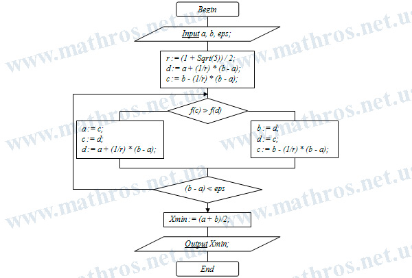
The golden section method is used to minimize a function of one variable on a given interval. In other words, we want to find the point on that interval where the function takes its smallest value. That may sound straightforward, but how can we do it efficiently and without unnecessary calculations? This is exactly where the golden section method is useful. It helps us narrow the search interval step by step instead of relying on guesswork. In this article, we will look at where the key numbers in the method come from and how the algorithm works on an interval.
Golden Section Method: The Ratio for Dividing an Interval
Let us begin with the basic idea. Suppose we have an interval \( [a,b] \) and we want to divide it with a point so that the two parts are unequal, but the division has a special property. Let \( c\in(a,b) \). This division is called “golden” when the ratio of the whole interval to the larger part is equal to the ratio of the larger part to the smaller part:
\[
\frac{b-a}{b-c}=\frac{b-c}{c-a}=r.
\]
Here, \( r \) is a constant that defines the division ratio. Now let us take an important step and express \( r \) from this condition.
Denote the lengths of the parts by
\[
L=b-a,\qquad x=b-c,\qquad L-x=c-a.
\]
Then the golden section condition becomes
\[
\frac{L}{x}=\frac{x}{L-x}.
\]
Cross-multiply:
\[
L \cdot (L-x)=x^2.
\]
Expand the brackets:
\[
L^2-L \cdot x=x^2.
\]
Move everything to one side:
\[
x^2+L \cdot x-L^2=0.
\]
This is a quadratic equation in \( x \). Solving it gives
\[
x=\frac{-L+\sqrt{L^2+4 \cdot L^2}}{2}=\frac{-L+\sqrt{5} \cdot L}{2}=L\cdot\frac{\sqrt{5}-1}{2}.
\]
So, the ratio \( \frac{x}{L} \) is
\[
\frac{x}{L}=\frac{\sqrt{5}-1}{2}.
\]
And the coefficient \( r \) is
\[
r=\frac{L}{x}=\frac{1}{\frac{\sqrt{5}-1}{2}}=\frac{2}{\sqrt{5}-1}=\frac{\sqrt{5}+1}{2}.
\]
That is,
\[
r=\frac{1+\sqrt{5}}{2}\approx 1.618.
\]
This is the number that determines how we place the points in the minimization algorithm. Neat, isn’t it?
Starting the Algorithm: Choosing Two Points and Making the First Comparison
Now let us move on to minimizing \( f(x) \) on the interval \( [a,b] \). We need two interior points so that we can compare the function values and discard part of the interval. Let us call them \( c \) and \( d \), where \( a<c<d<b \).

In the golden section method, these points are chosen so that they divide the interval in the “golden” ratio. The most convenient way to write them is in terms of \( r \):
\[
d=a+\frac{1}{r} \cdot (b-a),
\qquad
c=b-\frac{1}{r} \cdot (b-a).
\]
An important detail is that the points are symmetric relative to the midpoint in terms of length ratios, not actual distances. If you want the same formulas without \( r \), just substitute \( \frac{1}{r}=\frac{\sqrt{5}-1}{2} \):
\[
d=a+\frac{\sqrt{5}-1}{2} \cdot (b-a),
\qquad
c=b-\frac{\sqrt{5}-1}{2} \cdot (b-a).
\]
Next comes the step that defines the whole method: we compute and compare \( f(c) \) and \( f(d) \). At this point, the key question is simple: which part of the interval can we safely discard?
- If \( f(c)>f(d) \), then the minimum does not lie in \( [a,c] \). So we keep \( [a_1,b_1]=[c,b] \).
- If \( f(d)>f(c) \), then the minimum does not lie in \( [d,b] \). So we keep \( [a_1,b_1]=[a,d] \).
Why does this work? Because the method is applied to a unimodal function on \( [a,b] \), meaning it has only one minimum on that interval. So comparing the function values at two points tells us on which side the minimum lies. The logic is very practical: compare, discard, narrow the interval.
Golden Section Method: Interval Reduction, Stopping Criterion, and an Approximate Answer
Now comes the most satisfying part: after the first step, the interval becomes shorter, and it shrinks by the same constant factor each time. Let us see this directly from the formulas.
The initial length is
\[
L_0=b-a.
\]
After discarding part of the interval, the remaining interval has length
\[
L_1=b_1-a_1=\frac{1}{r} \cdot (b-a)=\frac{L_0}{r}.
\]
So, at each step, if we follow the method correctly, the length of the “interval of uncertainty” is multiplied by \( \frac{1}{r} \). After \( n \) steps, we get
\[
L_n=b_n-a_n=\frac{b-a}{r^n}.
\]
This gives us a direct estimate of how quickly the interval shrinks. And naturally, a practical question comes up: when should we stop?
Usually, we choose an accuracy \( \varepsilon>0 \) and stop the process when
\[
b_n-a_n<\varepsilon.
\]
Then, from the formula for \( L_n \), we get a condition for the number of steps:
\[
\frac{b-a}{r^n}<\varepsilon \quad\Longrightarrow\quad r^n>\frac{b-a}{\varepsilon}.
\]
Taking logarithms on both sides, in any base, though the natural logarithm is the most convenient, gives
\[
n>\frac{\ln\left(\frac{b-a}{\varepsilon}\right)}{\ln(r)}.
\]
So the number of iterations can be estimated in advance as the smallest integer \( n \) that satisfies this inequality. That is very convenient, because it tells you right away how many times you may need to evaluate \( f(x) \).
There is one more important point. Starting from the second step, we usually do not recompute both function values from scratch. One of the points carries over into the new interval, and its function value is already known. So at each later step, only one new computation of \( f(x) \) is often needed. That is exactly why this approach is so popular in numerical methods.
And how do we turn this into a specific answer?
After stopping, we have a small interval \( [a_n,b_n] \) that contains the minimum. A simple approximation is to take the midpoint:
\[
x^*\approx \frac{a_n+b_n}{2},
\]
or choose the point among the last ones where the function value is smaller. In the next section, this becomes much clearer through examples.
Practical Use of the Method: Step-by-Step Calculations
Now let us move on to actual calculations and see how the golden section method narrows the search interval with real numbers. Here, it is important not only to get the answer, but also to understand the logic behind each step. Then, in later problems, you will be able to repeat the algorithm on your own.
Example 1. Find the minimum of the function \( f(x)=(x-2)^2+1 \) on the interval \( [a,b]=[1,3] \) with accuracy \( \varepsilon=0.1 \) using the golden section method
Consider the function \( f(x)=(x-2)^2+1 \) on the interval \( [1,3] \). On this interval, it is unimodal because it has only one minimum near \( x=2 \). This means that comparing \( f(c) \) and \( f(d) \) allows us to safely discard part of the interval.
![Graph of the function f(x)=(x-2)^2+1 on the interval [1,3]](https://www.mathros.net.ua/en/wp-content/uploads/2026/03/golden-section-method2.jpg)
Take
\[
r=\frac{1+\sqrt{5}}{2}\approx 1.618,
\qquad
\frac{1}{r}\approx 0.618.
\]
Start with \( [a_0,b_0]=[1,3] \). Construct two points:
\[
\begin{gathered}
d_0=a_0+\frac{1}{r}(b_0-a_0)=1+0.618\cdot 2=2.236,
\\[6pt]
c_0=b_0-\frac{1}{r}(b_0-a_0)=3-0.618\cdot 2=1.764.
\end{gathered}
\]
Compute:
\[
\begin{gathered}
f(c_0)=(1.764-2)^2+1=1.056,
\\[6pt]
f(d_0)=(2.236-2)^2+1=1.056.
\end{gathered}
\]
We have equality, \( f(c_0)=f(d_0) \), so the interval can be narrowed in either of two symmetric ways. For definiteness, let us keep
\[
[a_1,b_1]=[1,2.236].
\]
Now here is an important detail. The point \( c_0=1.764 \) belongs to the new interval \( [a_1,b_1] \), so we can reuse it in the next step without recalculating the function value. That is,
\[
d_1=c_0=1.764,
\qquad
f(d_1)=f(c_0)=1.056.
\]
We find the second point using the formula:
\[
c_1=b_1-\frac{1}{r}(b_1-a_1)=2.236-0.618\cdot 1.236=1.472,
\]
and compute the new value:
\[
f(c_1)=(1.472-2)^2+1=1.279.
\]
Since \( f(c_1)>f(d_1) \), the minimum lies to the right, so
\[
[a_2,b_2]=[c_1,b_1]=[1.472,2.236].
\]
Next, we carry over the point whose function value is already known. In the new interval, the point \( d_1=1.764 \) remains, so
\[
c_2=d_1=1.764,
\qquad
f(c_2)=f(d_1)=1.056.
\]
Now we determine the other point:
\[
d_2=a_2+\frac{1}{r}(b_2-a_2)=1.472+0.618\cdot 0.764=1.944,
\]
and compute:
\[
f(d_2)=(1.944-2)^2+1=1.003.
\]
Since \( f(c_2)>f(d_2) \), we keep
\[
[a_3,b_3]=[c_2,b_2]=[1.764,2.236].
\]
Now, in this interval, the point \( d_2=1.944 \) remains, so
\[
c_3=d_2=1.944,
\qquad
f(c_3)=f(d_2)=1.003.
\]
We compute the other point:
\[
d_3=a_3+\frac{1}{r}(b_3-a_3)=1.764+0.618\cdot 0.472=2.056,
\]
and then:
\[
f(d_3)=(2.056-2)^2+1=1.003.
\]
Again, we have equality, \( f(c_3)=f(d_3) \), so for definiteness let us take
\[
[a_4,b_4]=[1.764,2.056].
\]
In this interval, the point \( c_3=1.944 \) remains, so
\[
d_4=c_3=1.944,
\qquad
f(d_4)=f(c_3)=1.003,
\]
and we find the other point:
\[
c_4=b_4-\frac{1}{r}(b_4-a_4)=2.056-0.618\cdot 0.292=1.876,
\]
then compute:
\[
f(c_4)=(1.876-2)^2+1=1.015.
\]
Since \( f(c_4)>f(d_4) \), we take
\[
[a_5,b_5]=[c_4,b_4]=[1.876,2.056].
\]
Next, the point \( d_4=1.944 \) remains, so
\[
c_5=d_4=1.944,
\qquad
f(c_5)=f(d_4)=1.003.
\]
We determine the other point:
\[
d_5=a_5+\frac{1}{r}(b_5-a_5)=1.876+0.618\cdot 0.180=1.987,
\]
and compute:
\[
f(d_5)=(1.987-2)^2+1=1.
\]
Since ( f(c_5)>f(d_5) ), we get
\[
[a_6,b_6]=[c_5,b_5]=[1.944,2.056].
\]
Now
\[
b_6-a_6=2.056-1.944=0.112,
\]
so we make one more step. The point \( d_5=1.987 \) remains in the interval, so
\[
c_6=d_5=1.987,
\qquad
f(c_6)=f(d_5)=1.
\]
We compute the other point:
\[
d_6=a_6+\frac{1}{r}(b_6-a_6)=1.944+0.618\cdot 0.112=2.013,
\]
and then:
\[
f(d_6)=(2.013-2)^2+1=1.
\]
Since the values are equal, the interval can once again be narrowed in either direction. For definiteness, let us take
\[
[a_7,b_7]=[1.944,2.013],
\qquad
b_7-a_7=0.069<0.1.
\]
So, the accuracy condition is satisfied. As a standard approximation of the minimum point, we take the midpoint:
\[
x^*\approx \frac{a_7+b_7}{2}=\frac{1.944+2.013}{2}=1.979.
\]
And if we use the smallest function value obtained so far, then the point
\[
x^*\approx 1.987,
\qquad
f(x^*)\approx 1
\]
is also a very good choice.
This agrees with the fact that the true minimum of this function is reached at \( x=2 \) and is equal to \( f_{\min}=1 \). So the method gave a close answer and did so by consistently and carefully narrowing the interval.
Example 2. Determine the number of iterations needed to find the minimum of the function \( f(x)=(x-2)^2+1 \) on the interval \( [a,b]=[1,3] \) with accuracy \( \varepsilon=0.1 \) using the golden section method
Now let us check whether the number of steps agrees with what we obtained in the previous example. We use the estimate
\[
n>\frac{\ln\left(\frac{b-a}{\varepsilon}\right)}{\ln(r)},
\qquad
r=\frac{1+\sqrt{5}}{2}.
\]
For \( [1,3] \), we have \( b-a=2 \), so
\[
\frac{b-a}{\varepsilon}=\frac{2}{0.1}=20,
\qquad
n>\frac{\ln(20)}{\ln(r)}.
\]
Take \( r\approx 1.618 \). Then \( \ln(20)\approx 2.996 \), \( \ln(1.618)\approx 0.481 \), so
\[
n>\frac{2.996}{0.481}\approx 6.225.
\]
Therefore, \( n=7 \) iterations are enough. This matches the practical result well: after the seventh step, we obtained an interval of length \( 0.069 \), which is already smaller than \( \varepsilon=0.1 \).
Where to Go Next: A Few More Minimization Methods
We have now worked through the golden section method and seen how it narrows the interval step by step. But what if you want other options and would like to understand when one method gives a better result than another? Here are several topics that naturally continue this article.
- Fibonacci Method: A Precise Step Plan — We will discuss how Fibonacci numbers define the sequence of checks and help plan the search for the minimum in advance.
- Dichotomy Method: Simple Interval Splitting — We will look at the idea of checking two points close to the midpoint and show how to narrow the search region quickly.
- Uniform Search: A Starting Approximation — We will explain how to move through the interval in equal steps, find the best subinterval, and build a good starting point for more accurate methods.
Golden Section Method in Code: Write Your Own Minimum Search
Now imagine that the flowchart below is not just a picture, but a ready-made plan for your own small learning project. Why not use it as a guide and write a compact program in your favorite programming language that finds the minimum value of a unimodal function using the golden section method?
This kind of project clearly shows how theory turns into a practical tool that you can run again and again on different functions. It is also a great way to test yourself. Do you understand the method equally well on paper and in code?