Eigenvectors of a Matrix: Computing Them Using the Danilevsky Method

The Danilevsky method allows us to find the eigenvectors of a matrix after the eigenvalues have already been found. This is important to understand right away. In this article, we will not construct the characteristic polynomial again or find its roots. Instead, we will focus on another question: how can we find the corresponding eigenvector when the eigenvalue is already known?

The advantage of this approach is that the original matrix is first reduced to a special form — the Frobenius matrix. For the Frobenius matrix, the eigenvector has a very simple form. After that, we only need to return to the original matrix using the transformation matrix. This is exactly the path we will follow step by step.

Eigenvectors of a Matrix: What Problem Do We Need to Solve?

Suppose we are given a square matrix \( A \). An eigenvector of this matrix is a nonzero vector \( x \) that, after being multiplied by the matrix \( A \), turns into a vector with the same direction.

In other words, for some number \( \lambda \), the equality \( A\cdot x=\lambda\cdot x \) holds. Here, \( \lambda \) is the eigenvalue, and \( x \) is the eigenvector that corresponds to it.

In our case, we assume that the eigenvalue \( \lambda \) has already been found. Therefore, the main task is not to calculate \( \lambda \), but to find a nonzero vector \( x \) that satisfies the equation \( A\cdot x=\lambda\cdot x \).

However, working directly with the matrix \( A \) is not always convenient. Why? Because the system for the coordinates of the eigenvector can have a complicated form. That is why the Danilevsky method uses an auxiliary Frobenius matrix. This matrix is similar to the matrix \( A \), but it has a much simpler structure.

So, the general idea is this: first, we find the eigenvector for the Frobenius matrix, and then, using the transformation matrix, we obtain the eigenvector of the original matrix.

Frobenius Matrix: Moving to a Convenient Form

In the Danilevsky method, the original matrix \( A \) is reduced to the Frobenius matrix \( P \) through a sequence of transformations. This matrix has a special form:

\[
P =
\begin{pmatrix}
p_1 & p_2 & p_3 & \dots & p_{n-1} & p_n \\
1 & 0 & 0 & \dots & 0 & 0 \\
0 & 1 & 0 & \dots & 0 & 0 \\
0 & 0 & 1 & \dots & 0 & 0 \\
\vdots & \vdots & \vdots & \ddots & \vdots & \vdots \\
0 & 0 & 0 & \dots & 1 & 0
\end{pmatrix}.
\]

This form is convenient because its elements have a clear structure. The first row contains the coefficients \( p_1,p_2,\dots,p_n \), while below it there are ones under the main diagonal.

The matrices \( A \) and \( P \) are similar. This means that they are connected by the equality:

\[
P=M^{-1}\cdot A\cdot M.
\]

Here, \( M \) is the transformation matrix. It combines all the transformations that were used to reduce the matrix \( A \) to the Frobenius matrix \( P \).

In this notation, the matrix \( M \) can be written as the product:

\[
M=M_1\cdot M_2\cdot M_3\cdot \dots \cdot M_{n-2}\cdot M_{n-1}.
\]

Since \( A \) and \( P \) are similar, they have the same eigenvalues. Therefore, if \( \lambda \) is an eigenvalue of the matrix \( A \), then it is also an eigenvalue of the matrix \( P \).

This is exactly what allows us to move to the next step: first, we find the eigenvector \( y \) for the matrix \( P \), and only after that do we obtain the required vector \( x \) for the matrix \( A \).

Vector of the Frobenius Matrix: How to Build the Solution

Let \( y=(y_1,y_2,y_3,\dots,y_n) \) be an eigenvector of the matrix \( P \) that corresponds to the eigenvalue \( \lambda \). Then the equality \( P\cdot y=\lambda\cdot y \) holds.

Now let us move the right-hand side of the equality to the left. We get a homogeneous system:

\[
(P-\lambda\cdot E)\cdot y=0,
\]

where \( E \) is the identity matrix.

For the Frobenius matrix, this system has a very convenient form:

\[
\begin{pmatrix}
p_1-\lambda & p_2 & p_3 & \dots & p_{n-1} & p_n \\
1 & -\lambda & 0 & \dots & 0 & 0 \\
0 & 1 & -\lambda & \dots & 0 & 0 \\
0 & 0 & 1 & \dots & 0 & 0 \\
\vdots & \vdots & \vdots & \ddots & \vdots & \vdots \\
0 & 0 & 0 & \dots & 1 & -\lambda
\end{pmatrix}
\cdot
\begin{pmatrix}
y_1\\
y_2\\
y_3\\
\vdots\\
y_n
\end{pmatrix}
=
\begin{pmatrix}
0\\
0\\
0\\
\vdots\\
0
\end{pmatrix}.
\]

After multiplying the matrix by the vector, we obtain the following system of equations:

\[
\begin{cases}
(p_1-\lambda)\cdot y_1+p_2\cdot y_2+p_3\cdot y_3+\dots+p_n\cdot y_n=0,\\
y_1-\lambda\cdot y_2=0,\\
y_2-\lambda\cdot y_3=0,\\
\vdots\\
y_{n-1}-\lambda\cdot y_n=0.
\end{cases}
\]

Now comes an important point. An eigenvector is defined up to a nonzero multiplier. In other words, if \( y \) is an eigenvector, then any vector \( c\cdot y \), where \( c\neq 0 \), will also be an eigenvector.

That is why one coordinate can be chosen freely. The most convenient choice is to set \( y_n=1 \). Then, from the last equation, we get \( y_{n-1}=\lambda \). Next, from the previous equation, we obtain \( y_{n-2}=\lambda^2 \). Continuing this process, we get:

\[
y_1=\lambda^{n-1}, \quad
y_2=\lambda^{n-2}, \quad
y_3=\lambda^{n-3}, \quad
\dots, \quad
y_n=1.
\]

Therefore, the eigenvector of the Frobenius matrix \( P \) that corresponds to the eigenvalue \( \lambda \) can be written as:

\[
y=
\begin{pmatrix}
\lambda^{n-1}\\
\lambda^{n-2}\\
\lambda^{n-3}\\
\vdots\\
1
\end{pmatrix}.
\]

But what happens to the first equation of the system? It still has an important role. This equation is directly connected with the characteristic equation of the matrix \( P \). Since \( \lambda \) is an eigenvalue of this matrix, the first equation is satisfied for the vector we have built.

So, the last equations give us the coordinates of the vector \( y \), while the first one confirms that this vector really corresponds to the eigenvalue \( \lambda \).

Eigenvectors of a Matrix: Returning to the Original Matrix

Now we have the eigenvector \( y \) of the Frobenius matrix \( P \). But the original problem is about the matrix \( A \), so we need to move from \( y \) to the eigenvector \( x \).

Let us use the connection between the matrices \( A \) and \( P \):

\[
P=M^{-1}\cdot A\cdot M.
\]

Since ( y ) is an eigenvector of the matrix \( P \), we have \( P\cdot y=\lambda\cdot y \). Now substitute \( M^{-1}\cdot A\cdot M \) instead of \( P \):

\[
M^{-1}\cdot A\cdot M\cdot y=\lambda\cdot y.
\]

Now multiply both sides of the equality on the left by the matrix \( M \). We get:

\[
A\cdot M\cdot y=\lambda \cdot M\cdot y.
\]

This equality has the same form as the equation for an eigenvector of the matrix \( A \). Therefore, the vector \( M\cdot y \) is an eigenvector of the matrix \( A \).

So, the required eigenvector is written as:

\[
x=M\cdot y.
\]

Since the vector \( y \) has already been found, we get the final formula:

\[
x
=
M\cdot
\begin{pmatrix}
\lambda^{n-1}\\
\lambda^{n-2}\\
\lambda^{n-3}\\
\vdots\\
1
\end{pmatrix}.
\]

So, the scheme for finding an eigenvector using the Danilevsky method is as follows. First, we use the known eigenvalue \( \lambda \). Then we construct the eigenvector of the Frobenius matrix:

\[
y=
\begin{pmatrix}
\lambda^{n-1}\\
\lambda^{n-2}\\
\lambda^{n-3}\\
\vdots\\
1
\end{pmatrix}.
\]

After that, we multiply it by the transformation matrix \( M \) and obtain the eigenvector of the original matrix:

\[
x=M\cdot y.
\]

Thus, the Danilevsky method allows us not only to find eigenvalues but also to build the corresponding eigenvectors. The main thing is to remember the sequence: first, we work with the Frobenius matrix, and then we return to the original matrix through the transformation matrix.

Practical Part: How to Find Eigenvectors of a Matrix Using the Danilevsky Method

Now let us apply the described scheme to specific matrices. In each example, the eigenvalues are already given, so we do not need to find the characteristic polynomial. Our task is to construct the eigenvectors using the Frobenius matrix and the transformation matrix.

Example 1. Using the Danilevsky method, find the eigenvectors of the matrix
\[
A=
\begin{pmatrix}
2 & 1 \\
3 & 4
\end{pmatrix},
\]
if its eigenvalues are
\[
\lambda_1=1,
\qquad
\lambda_2=5.
\]

We have a \( 2\times2 \) matrix. Therefore, after the Danilevsky transformation, it should be reduced to a Frobenius matrix of the form

\[
P=
\begin{pmatrix}
p_1 & p_2\\
1 & 0
\end{pmatrix}.
\]

The transformation matrix is built so that, after the transformation \( P=M_1^{-1}\cdot A\cdot M_1 \), the bottom row of the Frobenius matrix has the form \( (1,0) \). For this matrix, the corresponding transformation matrix is

\[
M_1=
\begin{pmatrix}
\dfrac{1}{3} & -\dfrac{4}{3}\\
0 & 1
\end{pmatrix}.
\]

Then

\[
P=M_1^{-1}\cdot A\cdot M_1.
\]

After multiplication, we get

\[
P=
\begin{pmatrix}
6 & -5\\
1 & 0
\end{pmatrix}.
\]

So, the original matrix \( A \) has been reduced to the Frobenius matrix \( P \).

For a \( 2\times2 \) matrix, the eigenvector of the matrix \( P \) that corresponds to the eigenvalue \( \lambda \) has the form

\[
y=
\begin{pmatrix}
\lambda\\
1
\end{pmatrix}.
\]

Now we find the eigenvector of the original matrix \( A \) using the formula

\[
x=M_1\cdot y.
\]

First, consider the eigenvalue \( \lambda_1=1 \). For it, we have

\[
y_1=
\begin{pmatrix}
1\\
1
\end{pmatrix}.
\]

Then

\[
x_1=
M_1\cdot y_1
=
\begin{pmatrix}
\dfrac{1}{3} & -\dfrac{4}{3}\\
0 & 1
\end{pmatrix}
\cdot
\begin{pmatrix}
1\\
1
\end{pmatrix}.
\]

Now perform the multiplication:

\[
x_1=
\begin{pmatrix}
\dfrac{1}{3}-\dfrac{4}{3}\\
1
\end{pmatrix}
=
\begin{pmatrix}
-1\\
1
\end{pmatrix}.
\]

Therefore, the eigenvalue \( \lambda_1=1 \) corresponds to the eigenvector

\[
x_1=
\begin{pmatrix}
-1\\
1
\end{pmatrix}.
\]

Let us check the result:

\[
A\cdot x_1
=
\begin{pmatrix}
2 & 1\\
3 & 4
\end{pmatrix}
\cdot
\begin{pmatrix}
-1\\
1
\end{pmatrix}
=
\begin{pmatrix}
-1\\
1
\end{pmatrix}.
\]

Since

\[
1\cdot x_1
=
1\cdot
\begin{pmatrix}
-1\\
1
\end{pmatrix}
=
\begin{pmatrix}
-1\\
1
\end{pmatrix},
\]

this confirms the result.

Now consider the eigenvalue \( \lambda_2=5 \). For it,

\[
y_2=
\begin{pmatrix}
5\\
1
\end{pmatrix}.
\]

Then

\[
x_2=
M_1\cdot y_2
=
\begin{pmatrix}
\dfrac{1}{3} & -\dfrac{4}{3}\\
0 & 1
\end{pmatrix}
\cdot
\begin{pmatrix}
5\\
1
\end{pmatrix}.
\]

Hence,

\[
x_2=
\begin{pmatrix}
\dfrac{5}{3}-\dfrac{4}{3}\\
1
\end{pmatrix}
=
\begin{pmatrix}
\dfrac{1}{3}\\
1
\end{pmatrix}.
\]

An eigenvector can be multiplied by any nonzero number. So, to avoid fractions, let us multiply it by \( 3 \). We get

\[
x_2=
\begin{pmatrix}
1\\
3
\end{pmatrix}.
\]

Let us check:

\[
A\cdot x_2
=
\begin{pmatrix}
2 & 1\\
3 & 4
\end{pmatrix}
\cdot
\begin{pmatrix}
1\\
3
\end{pmatrix}
=
\begin{pmatrix}
5\\
15
\end{pmatrix}.
\]

Also,

\[
5\cdot x_2
=
5\cdot
\begin{pmatrix}
1\\
3
\end{pmatrix}
=
\begin{pmatrix}
5\\
15
\end{pmatrix}.
\]

So, the result is correct.

Thus, for the given matrix, we have

\[
\begin{gathered}
\lambda_1=1:\qquad
x_1=\begin{pmatrix}
-1\\
1
\end{pmatrix},
\\[4pt]
\lambda_2=5:\qquad
x_2=\begin{pmatrix}
1\\
3
\end{pmatrix}.
\end{gathered}
\]

Example 2. Using the Danilevsky method, find the eigenvectors of the matrix
\[
A=
\begin{pmatrix}
3 & 0 & 0 \\
1 & 1 & 2 \\
0 & 1 & 0
\end{pmatrix},
\]
if its eigenvalues are
\[
\lambda_1=3,
\qquad
\lambda_2=2,
\qquad
\lambda_3=-1.
\]

We have a \( 3\times3 \) matrix. Therefore, after applying the Danilevsky method, it is reduced to a Frobenius matrix of the form

\[
P=
\begin{pmatrix}
p_1 & p_2 & p_3\\
1 & 0 & 0\\
0 & 1 & 0
\end{pmatrix}.
\]

The transformation matrix \( M \) is built according to the rules of the Danilevsky method so that, after the transformation \( P=M^{-1}\cdot A\cdot M \), we obtain exactly the Frobenius matrix. For this matrix, the corresponding transformation matrix is

\[
M=
\begin{pmatrix}
1 & -1 & -2\\
0 & 1 & 0\\
0 & 0 & 1
\end{pmatrix}.
\]

Then

\[
P=M^{-1}\cdot A\cdot M.
\]

After the calculations, we get

\[
P=
\begin{pmatrix}
4 & -1 & -6\\
1 & 0 & 0\\
0 & 1 & 0
\end{pmatrix}.
\]

So, the matrix \( A \) has been reduced to the Frobenius matrix.

For a \( 3\times3 \) matrix, the eigenvector of the matrix \( P \) that corresponds to the eigenvalue \( \lambda \) has the form

\[
y=
\begin{pmatrix}
\lambda^2\\
\lambda\\
1
\end{pmatrix}.
\]

Now we find the eigenvector of the original matrix \( A \) using the formula

\[
x=M\cdot y.
\]

Substitute the matrix \( M \) and the vector \( y \):

\[
x=
\begin{pmatrix}
1 & -1 & -2\\
0 & 1 & 0\\
0 & 0 & 1
\end{pmatrix}
\cdot
\begin{pmatrix}
\lambda^2\\
\lambda\\
1
\end{pmatrix}.
\]

After multiplication, we get the general form of the eigenvector:

\[
x=
\begin{pmatrix}
\lambda^2-\lambda-2\\
\lambda\\
1
\end{pmatrix}.
\]

Now substitute the given eigenvalues.

For \( \lambda_1=3 \):

\[
x_1=
\begin{pmatrix}
3^2-3-2\\
3\\
1
\end{pmatrix}
=
\begin{pmatrix}
4\\
3\\
1
\end{pmatrix}.
\]

Let us verify the result:

\[
A\cdot x_1
=
\begin{pmatrix}
3 & 0 & 0 \\
1 & 1 & 2 \\
0 & 1 & 0
\end{pmatrix}
\cdot
\begin{pmatrix}
4\\
3\\
1
\end{pmatrix}
=
\begin{pmatrix}
12\\
9\\
3
\end{pmatrix}.
\]

Also,

\[
3\cdot x_1
=
3\cdot
\begin{pmatrix}
4\\
3\\
1
\end{pmatrix}
=
\begin{pmatrix}
12\\
9\\
3
\end{pmatrix}.
\]

So, the vector we found really corresponds to the eigenvalue \( \lambda_1=3 \).

For \( \lambda_2=2 \):

\[
x_2=
\begin{pmatrix}
2^2-2-2\\
2\\
1
\end{pmatrix}
=
\begin{pmatrix}
0\\
2\\
1
\end{pmatrix}.
\]

Let us check:

\[
A\cdot x_2
=
\begin{pmatrix}
3 & 0 & 0 \\
1 & 1 & 2 \\
0 & 1 & 0
\end{pmatrix}
\cdot
\begin{pmatrix}
0\\
2\\
1
\end{pmatrix}
=
\begin{pmatrix}
0\\
4\\
2
\end{pmatrix}.
\]

Also,

\[
2\cdot x_2
=
2\cdot
\begin{pmatrix}
0\\
2\\
1
\end{pmatrix}
=
\begin{pmatrix}
0\\
4\\
2
\end{pmatrix}.
\]

So, the equality holds, which means that the vector \( x_2 \) has been found correctly.

For \( \lambda_3=-1 \):

\[
x_3=
\begin{pmatrix}
(-1)^2-(-1)-2\\
-1\\
1
\end{pmatrix}
=
\begin{pmatrix}
0\\
-1\\
1
\end{pmatrix}.
\]

Let us check:

\[
A\cdot x_3
=
\begin{pmatrix}
3 & 0 & 0 \\
1 & 1 & 2 \\
0 & 1 & 0
\end{pmatrix}
\cdot
\begin{pmatrix}
0\\
-1\\
1
\end{pmatrix}
=
\begin{pmatrix}
0\\
1\\
-1
\end{pmatrix}.
\]

Also,

\[
-1\cdot x_3
=
-1\cdot
\begin{pmatrix}
0\\
-1\\
1
\end{pmatrix}
=
\begin{pmatrix}
0\\
1\\
-1
\end{pmatrix}.
\]

Therefore, the obtained vector is an eigenvector for \( \lambda_3=-1 \).

Thus, for the given matrix \( A \), we have obtained the following eigenvectors:

\[
\begin{gathered}
\lambda_1=3:\qquad
x_1=\begin{pmatrix}
4\\
3\\
1
\end{pmatrix},
\\[4pt]
\lambda_2=2:\qquad
x_2=\begin{pmatrix}
0\\
2\\
1
\end{pmatrix},
\\[4pt]
\lambda_3=-1:\qquad
x_3=\begin{pmatrix}
0\\
-1\\
1
\end{pmatrix}.
\end{gathered}
\]

Example 3. Using the Danilevsky method, find the eigenvectors of the matrix
\[
A=
\begin{pmatrix}
-4 & -1 & -3 \\
4 & 3 & 6 \\
0 & -1 & -2
\end{pmatrix},
\]
if its eigenvalues are
\[
\lambda_1=1,
\qquad
\lambda_2=-2,
\qquad
\lambda_3=-2.
\]

In this example, the eigenvalue \( \lambda=-2 \) is repeated twice, so it is a multiple eigenvalue. However, the multiplicity of an eigenvalue does not guarantee that two different linearly independent eigenvectors will appear. Therefore, after the calculations, it is worth checking whether we get a new eigenvector direction or the same one.

First, reduce the matrix \( A \) to the Frobenius matrix. At the first step, use the matrix

\[
M_2=
\begin{pmatrix}
1 & 0 & 0\\
0 & -1 & -2\\
0 & 0 & 1
\end{pmatrix}.
\]

Then

\[
A^{(1)}=M_2^{-1}\cdot A\cdot M_2.
\]

After multiplication, we have

\[
A^{(1)}
=
\begin{pmatrix}
-4 & 1 & -1\\
-4 & 1 & 0\\
0 & 1 & 0
\end{pmatrix}.
\]

At the second step, use the matrix

\[
M_1=
\begin{pmatrix}
-\dfrac{1}{4} & \dfrac{1}{4} & 0\\
0 & 1 & 0\\
0 & 0 & 1
\end{pmatrix}.
\]

Then the Frobenius matrix is found as follows:

\[
P=M_1^{-1}\cdot A^{(1)}\cdot M_1.
\]

We get

\[
P=
\begin{pmatrix}
-3 & 0 & 4\\
1 & 0 & 0\\
0 & 1 & 0
\end{pmatrix}.
\]

The final transformation matrix is

\[
M=M_2\cdot M_1.
\]

That is,

\[
M=
\begin{pmatrix}
1 & 0 & 0\\
0 & -1 & -2\\
0 & 0 & 1
\end{pmatrix}
\cdot
\begin{pmatrix}
-\dfrac{1}{4} & \dfrac{1}{4} & 0\\
0 & 1 & 0\\
0 & 0 & 1
\end{pmatrix}.
\]

After multiplication, we have

\[
M=
\begin{pmatrix}
-\dfrac{1}{4} & \dfrac{1}{4} & 0\\
0 & -1 & -2\\
0 & 0 & 1
\end{pmatrix}.
\]

For a \( 3\times3 \) matrix, the eigenvector of the Frobenius matrix has the form

\[
y=
\begin{pmatrix}
\lambda^2\\
\lambda\\
1
\end{pmatrix}.
\]

Therefore, the eigenvector of the original matrix \( A \) is found by the formula

\[
x=M\cdot y.
\]

Substitute \( M \) and \( y \):

\[
x=
\begin{pmatrix}
-\dfrac{1}{4} & \dfrac{1}{4} & 0\\
0 & -1 & -2\\
0 & 0 & 1
\end{pmatrix}
\cdot
\begin{pmatrix}
\lambda^2\\
\lambda\\
1
\end{pmatrix}.
\]

After multiplication, we get

\[
x=
\begin{pmatrix}
-\dfrac{\lambda^2}{4}+\dfrac{\lambda}{4}\\
-\lambda-2\\
1
\end{pmatrix}.
\]

Or, more briefly,

\[
x=
\begin{pmatrix}
\dfrac{-\lambda^2+\lambda}{4}\\
-\lambda-2\\
1
\end{pmatrix}.
\]

Now substitute the eigenvalues.

For \( \lambda_1=1 \):

\[
x_1=
\begin{pmatrix}
\dfrac{-1^2+1}{4}\\
-1-2\\
1
\end{pmatrix}.
\]

Hence,

\[
x_1=
\begin{pmatrix}
0\\
-3\\
1
\end{pmatrix}.
\]

Let us check:

\[
A\cdot x_1
=
\begin{pmatrix}
-4 & -1 & -3 \\
4 & 3 & 6 \\
0 & -1 & -2
\end{pmatrix}
\cdot
\begin{pmatrix}
0\\
-3\\
1
\end{pmatrix}
=
\begin{pmatrix}
0\\
-3\\
1
\end{pmatrix}.
\]

Since

\[
1\cdot x_1
=
1\cdot
\begin{pmatrix}
0\\
-3\\
1
\end{pmatrix}
=
\begin{pmatrix}
0\\
-3\\
1
\end{pmatrix},
\]

the eigenvector for \( \lambda_1=1 \) has been found correctly.

Now consider the eigenvalue \( \lambda_2=-2 \). Substitute it into the general formula:

\[
x_2=
\begin{pmatrix}
\dfrac{-(-2)^2+(-2)}{4}\\
-(-2)-2\\
1
\end{pmatrix}.
\]

We get

\[
x_2=
\begin{pmatrix}
-\dfrac{3}{2}\\
0\\
1
\end{pmatrix}.
\]

To avoid fractions, multiply this vector by \( 2 \). We have

\[
x_2=
\begin{pmatrix}
-3\\
0\\
2
\end{pmatrix}.
\]

Let us check:

\[
A\cdot x_2
=
\begin{pmatrix}
-4 & -1 & -3 \\
4 & 3 & 6 \\
0 & -1 & -2
\end{pmatrix}
\cdot
\begin{pmatrix}
-3\\
0\\
2
\end{pmatrix}
=
\begin{pmatrix}
6\\
0\\
-4
\end{pmatrix}.
\]

Also,

\[
-2\cdot x_2
=
-2\cdot
\begin{pmatrix}
-3\\
0\\
2
\end{pmatrix}
=
\begin{pmatrix}
6\\
0\\
-4
\end{pmatrix}.
\]

So, the eigenvector for the eigenvalue \( \lambda_2=-2 \) has also been found correctly.

Now pay attention to \( \lambda_3=-2 \). This is the same eigenvalue that has already been considered. If we substitute \( \lambda=-2 \) into the formula for \( x \) again, we get the same vector:

\[
x_3=
\begin{pmatrix}
-3\\
0\\
2
\end{pmatrix}.
\]

This means that, for the multiple eigenvalue \( \lambda=-2 \), this example gives only one direction of the eigenvector. In other words, the value \( \lambda=-2 \) appears twice among the eigenvalues, but it does not give two different linearly independent eigenvectors.

Therefore, in this case, for the matrix \( A \), we have

\[
\begin{gathered}
\lambda_1=1:\qquad
x_1=\begin{pmatrix}
0\\
-3\\
1
\end{pmatrix},
\\[4pt]
\lambda_2=-2:\qquad
x_2=\begin{pmatrix}
-3\\
0\\
2
\end{pmatrix},
\\[4pt]
\lambda_3=-2:\qquad
x_3=\begin{pmatrix}
-3\\
0\\
2
\end{pmatrix}.
\end{gathered}
\]

What to Read Next: Three Topics to Continue With

After the Danilevsky method, it is useful to look at other approaches to working with eigenvalues and eigenvectors. This will make it easier to see how the same problem can be solved by different methods.

1. Characteristic Determinant: Eigenvalues and Eigenvectors of a Matrix — This article will show how eigenvalues are found using the characteristic determinant and how the corresponding eigenvectors of a matrix are then built.
2. Krylov Method: How to Find Eigenvalues of a Matrix — This article will show how the Krylov method helps build the characteristic equation and find the eigenvalues of a matrix.
3. Eigenvectors: Continuing the Krylov Method — This article will explain how, after finding eigenvalues using the Krylov method, we can move on to building eigenvectors.

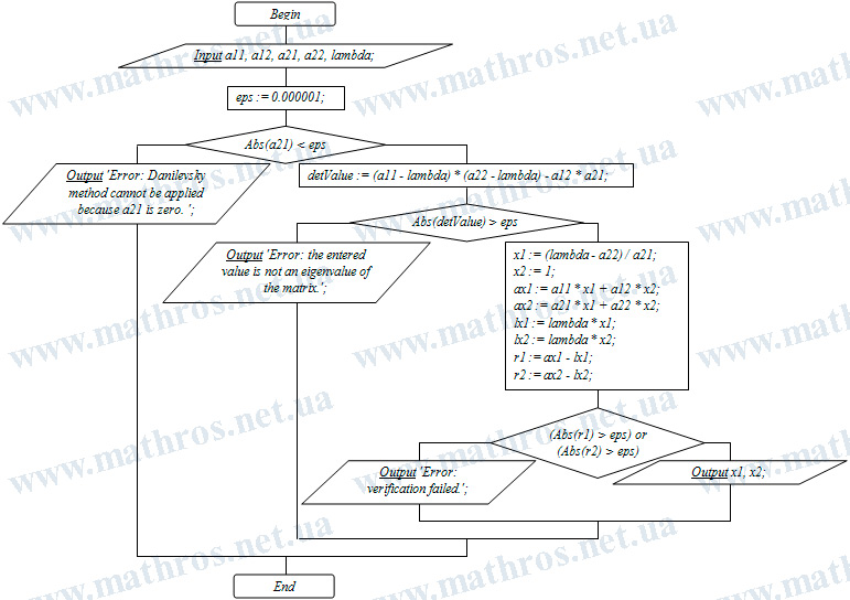
Eigenvectors of a Matrix: From Flowchart to Program

If you enjoy programming, this stage may become the most interesting part of the whole topic. After all, the Danilevsky method is no longer just a set of formulas on paper. It becomes a ready-made algorithm that can be implemented in Pascal, Python, C++, Java, or any other programming language you feel comfortable using.

Try to study the flowchart carefully, follow each step, and turn it into program code: entering the matrix, checking the eigenvalue, calculating the coordinates of the eigenvector, and verifying the correctness of the result. Isn’t it interesting to see how a mathematical method turns into a real working tool?