Eigenvalues of a matrix can be found not only by directly calculating the characteristic determinant. One convenient approach is the Faddeev method. It is considered an exact computational method and is closely related to the Leverrier method.
Its main advantage is the step-by-step structure of the calculations. First, auxiliary matrices are formed. Then, using their traces, the coefficients of the characteristic polynomial are found. After that, the eigenvalues of the matrix are determined. In addition, the Faddeev method can be used to find the inverse matrix and eigenvectors.
Eigenvalues of a Matrix Using the Faddeev Method: Main Idea
The Faddeev method can be viewed as a modification of the Leverrier method. In the Leverrier method, powers of a matrix are used to find the coefficients of the characteristic polynomial:
\[
A,\ A^2,\ \dots,\ A^n.
\]
The Faddeev method works differently. Instead of directly calculating powers of the matrix, it constructs auxiliary matrices. This sequence gradually leads to the coefficients of the characteristic polynomial.
Let a square matrix \( A \) of order \( n \) be given:
\[
A=
\begin{pmatrix}
a_{11} & a_{12} & \dots & a_{1n}\\
a_{21} & a_{22} & \dots & a_{2n}\\
\vdots & \vdots & \ddots & \vdots\\
a_{n1} & a_{n2} & \dots & a_{nn}
\end{pmatrix}.
\]
We need to find its eigenvalues. Where should we start? First, we need to construct the characteristic polynomial.
In the Faddeev method, it is convenient to write it as follows:
\[
D(\lambda)=\lambda^n-\sigma_1\cdot\lambda^{n-1}-\sigma_2\cdot\lambda^{n-2}-\dots-\sigma_{n-1}\cdot\lambda-\sigma_n.
\]
Then the eigenvalues of the matrix are found from the characteristic equation:
\[
D(\lambda)=0.
\]
So, the task of the Faddeev method is to find the coefficients
\[
\sigma_1,\sigma_2,\dots,\sigma_n.
\]
After that, all that remains is to solve the characteristic equation. Its roots will be the eigenvalues of the matrix \( A \).
Faddeev Method: Construction of Auxiliary Matrices
Now let us move on to the algorithm itself. Let \( I \) be the identity matrix of the same order as the matrix \( A \):
\[
I=
\begin{pmatrix}
1 & 0 & \dots & 0\\
0 & 1 & \dots & 0\\
\vdots & \vdots & \ddots & \vdots\\
0 & 0 & \dots & 1
\end{pmatrix}.
\]
In the Faddeev method, the matrices
\[
A_1,A_2,\dots,A_n
\]
and
\[
B_1,B_2,\dots,B_n
\]
are constructed step by step.
Let us start with the first step. First, we take the original matrix:
\[
A_1=A.
\]
Then, using the trace of the matrix \( A_1 \), we find the number \( q_1 \):
\[
q_1=tr(A_1).
\]
After that, we construct the first auxiliary matrix:
\[
B_1=A_1-q_1\cdot I.
\]
Why do we need the matrix \( B_1 \)? It is used to construct the next matrix \( A_2 \). In other words, the first step does not complete the calculation. It prepares the transition to the next stage.
Now we move on to the second step. This time, we multiply the original matrix \( A \) by the matrix \( B_1 \) that has already been found:
\[
A_2=A\cdot B_1.
\]
Next, we find the number \( q_2 \). To do this, we take the trace of the matrix \( A_2 \) and divide it by the step number:
\[
q_2=\frac{tr(A_2)}{2}.
\]
After that, we construct the second auxiliary matrix:
\[
B_2=A_2-q_2\cdot I.
\]
The matrix \( B_2 \), just like \( B_1 \), is needed to continue the algorithm. It will be used in the next step when constructing the matrix \( A_3 \).
After the second step, the pattern becomes clear. Each subsequent step follows the same principle: a new matrix \( A_k \) is formed using the previous matrix \( B_{k-1} \), the number \( q_k \) is found from the trace of the matrix \( A_k \), and the matrix \( B_k \) prepares the next step.
In the general case, if the matrix \( B_{k-1} \) has already been found, then for step \( k \) we have:
\[
A_k=A\cdot B_{k-1},\qquad q_k=\frac{tr(A_k)}{k},\qquad B_k=A_k-q_k\cdot I,
\]
where \( k=3,4,\dots,n \).
The trace of a matrix is the sum of the elements on its main diagonal. If, at some step, the matrix \( A_k \) has the form
\[
A_k=
\begin{pmatrix}
a_{11}^{(k)} & a_{12}^{(k)} & \dots & a_{1n}^{(k)}\\
a_{21}^{(k)} & a_{22}^{(k)} & \dots & a_{2n}^{(k)}\\
\vdots & \vdots & \ddots & \vdots\\
a_{n1}^{(k)} & a_{n2}^{(k)} & \dots & a_{nn}^{(k)}
\end{pmatrix},
\]
then, in the general case, its trace is calculated as follows:
\[
tr(A_k)=a_{11}^{(k)}+a_{22}^{(k)}+\dots+a_{nn}^{(k)}.
\]
The numbers
\[
q_1,q_2,\dots,q_n
\]
play a key role in the algorithm. After the construction of the matrices is completed, they are used as the coefficients of the characteristic polynomial, taking into account the chosen form of this polynomial.
So, in the second section, we have obtained the computational scheme of the Faddeev method itself. Now we only need to understand how to move from the numbers \( q_k \) to the characteristic polynomial and the eigenvalues.
Characteristic Polynomial: Transition to Eigenvalues of a Matrix
After the construction of the auxiliary matrices is completed, we have the numbers
\[
q_1,q_2,\dots,q_n.
\]
Now they define the coefficients of the characteristic polynomial:
\[
\sigma_1=q_1,\qquad \sigma_2=q_2,\qquad \dots,\qquad \sigma_n=q_n.
\]
Or, in short:
\[
\sigma_k=q_k,\qquad k=1,2,\dots,n.
\]
Therefore, the characteristic polynomial of the matrix \( A \) is written in the form
\[
D(\lambda)=\lambda^n-\sigma_1\cdot\lambda^{n-1}-\sigma_2\cdot\lambda^{n-2}-\dots-\sigma_{n-1}\cdot\lambda-\sigma_n.
\]
Taking into account the numbers \( q_1,q_2,\dots,q_n \) that we have found, we get
\[
D(\lambda)=\lambda^n-q_1\cdot\lambda^{n-1}-q_2\cdot\lambda^{n-2}-\dots-q_{n-1}\cdot\lambda-q_n.
\]
Next, we solve the characteristic equation:
\[
D(\lambda)=0.
\]
Its roots
\[
\lambda_1,\lambda_2,\dots,\lambda_n
\]
are the eigenvalues of the matrix \( A \).
So, it is important not to mix two stages. The Faddeev method first gives the coefficients of the characteristic polynomial. Only after that are the eigenvalues found as the roots of the characteristic equation.
Besides finding eigenvalues, as already mentioned, the Faddeev method has one more useful property. If the matrix \( A \) is nonsingular, that is,
\[
\det A\neq 0,
\]
then we can find the inverse matrix:
\[
A^{-1}=\frac{B_{n-1}}{\sigma_n}.
\]
In this formula, the same sign of the coefficient \( \sigma_n \) is used as in the characteristic polynomial written above. This is important because different sources may write the characteristic polynomial using a different sign convention.
The Faddeev method also makes it possible to find eigenvectors. If \( \lambda_i \) is an eigenvalue of the matrix \( A \), then we construct the matrix
\[
R_i=\lambda_i^{n-1}\cdot I+\lambda_i^{n-2}\cdot B_1+\dots+\lambda_i\cdot B_{n-2}+B_{n-1}.
\]
Each nonzero column of the matrix \( R_i \) can be taken as an eigenvector corresponding to the eigenvalue \( \lambda_i \).
Thus, the Faddeev method gives a step-by-step scheme for working with a matrix. First, the matrices \( A_k \) and \( B_k \) are constructed. Then the numbers \( q_k \) are found from the traces of these matrices. After that, the characteristic polynomial is formed, and its roots give the eigenvalues of the matrix.
Practical Part: How to Find Eigenvalues of a Matrix by the Faddeev Method
Now let us see how the Faddeev method works with specific matrices. We will start with a second-order matrix and then gradually move on to third-order and fourth-order matrices. In each example, we will construct auxiliary matrices, find the coefficients of the characteristic polynomial, and then move on to the eigenvalues.
Example 1. Find the eigenvalues of the matrix
\[
A=
\begin{pmatrix}
2 & 1\\
0 & 3
\end{pmatrix}.
\]
We have a second-order matrix, so we need to perform two steps. We start with the matrix
\[
A_1=A=
\begin{pmatrix}
2 & 1\\
0 & 3
\end{pmatrix}.
\]
We find the number \( q_1 \) from the trace of the matrix \( A_1 \):
\[
q_1=tr(A_1)=2+3=5.
\]
Now we construct the matrix \( B_1 \):
\[
B_1=A_1-q_1\cdot I.
\]
Substitute the matrices:
\[
B_1=
\begin{pmatrix}
2 & 1\\
0 & 3
\end{pmatrix}
–
5\cdot
\begin{pmatrix}
1 & 0\\
0 & 1
\end{pmatrix}.
\]
Therefore,
\[
B_1=
\begin{pmatrix}
-3 & 1\\
0 & -2
\end{pmatrix}.
\]
Now we move on to the second step. We find the matrix \( A_2 \). To do this, we multiply the original matrix \( A \) by the matrix \( B_1 \):
\[
A_2=A\cdot B_1.
\]
That is,
\[
A_2=
\begin{pmatrix}
2 & 1\\
0 & 3
\end{pmatrix}
\cdot
\begin{pmatrix}
-3 & 1\\
0 & -2
\end{pmatrix}.
\]
After multiplication, we get
\[
A_2=
\begin{pmatrix}
-6 & 0\\
0 & -6
\end{pmatrix}.
\]
Now we find the number \( q_2 \):
\[
q_2=\frac{tr(A_2)}{2}=\frac{-6+(-6)}{2}=-6.
\]
So,
\[
q_1=5,\qquad q_2=-6.
\]
For a second-order matrix, the characteristic polynomial has the form
\[
D(\lambda)=\lambda^2-q_1\cdot\lambda-q_2.
\]
Substitute the values we have found:
\[
D(\lambda)=\lambda^2-5\cdot\lambda-(-6).
\]
That is,
\[
D(\lambda)=\lambda^2-5\cdot\lambda+6.
\]
We solve the characteristic equation:
\[
\lambda^2-5\cdot\lambda+6=0.
\]
Let us factor the left-hand side:
\[
(\lambda-2)\cdot(\lambda-3)=0.
\]
From this, we get the eigenvalues:
\[
\lambda_1=2,\qquad \lambda_2=3.
\]
Example 2. Find the eigenvalues of the matrix
\[
A=
\begin{pmatrix}
1 & 1 & 0\\
0 & 2 & 1\\
0 & 0 & 3
\end{pmatrix}.
\]
This is a third-order matrix, so we need to find the numbers \( q_1,\ q_2,\ q_3 \).
We start with the first step:
\[
A_1=A=
\begin{pmatrix}
1 & 1 & 0\\
0 & 2 & 1\\
0 & 0 & 3
\end{pmatrix}.
\]
We find the trace of the matrix \( A_1 \):
\[
q_1=tr(A_1)=1+2+3=6.
\]
We construct the matrix \( B_1 \):
\[
B_1=A_1-q_1\cdot I.
\]
Substitute the matrices:
\[
B_1=
\begin{pmatrix}
1 & 1 & 0\\
0 & 2 & 1\\
0 & 0 & 3
\end{pmatrix}
–
6\cdot
\begin{pmatrix}
1 & 0 & 0\\
0 & 1 & 0\\
0 & 0 & 1
\end{pmatrix}.
\]
Therefore,
\[
B_1=
\begin{pmatrix}
-5 & 1 & 0\\
0 & -4 & 1\\
0 & 0 & -3
\end{pmatrix}.
\]
Now we move on to the second step. We find the matrix \( A_2 \). To do this, we multiply the matrix \( A \) by the matrix \( B_1 \):
\[
A_2=A\cdot B_1.
\]
That is,
\[
A_2=
\begin{pmatrix}
1 & 1 & 0\\
0 & 2 & 1\\
0 & 0 & 3
\end{pmatrix}
\cdot
\begin{pmatrix}
-5 & 1 & 0\\
0 & -4 & 1\\
0 & 0 & -3
\end{pmatrix}.
\]
After multiplication, we get
\[
A_2=
\begin{pmatrix}
-5 & -3 & 1\\
0 & -8 & -1\\
0 & 0 & -9
\end{pmatrix}.
\]
We find the number \( q_2 \):
\[
q_2=\frac{tr(A_2)}{2}=\frac{-5+(-8)+(-9)}{2}=\frac{-22}{2}=-11.
\]
Now we construct the matrix \( B_2 \):
\[
B_2=A_2-q_2\cdot I.
\]
Since \( q_2=-11 \), we have
\[
B_2=A_2-(-11)\cdot I.
\]
Substitute the matrices:
\[
B_2=
\begin{pmatrix}
-5 & -3 & 1\\
0 & -8 & -1\\
0 & 0 & -9
\end{pmatrix}
–
(-11)\cdot
\begin{pmatrix}
1 & 0 & 0\\
0 & 1 & 0\\
0 & 0 & 1
\end{pmatrix}.
\]
Therefore,
\[
B_2=
\begin{pmatrix}
6 & -3 & 1\\
0 & 3 & -1\\
0 & 0 & 2
\end{pmatrix}.
\]
Now we move on to the third step. We find the matrix \( A_3 \). To do this, we multiply the matrix \( A \) by the matrix \( B_2 \):
\[
A_3=A\cdot B_2.
\]
That is,
\[
A_3=
\begin{pmatrix}
1 & 1 & 0\\
0 & 2 & 1\\
0 & 0 & 3
\end{pmatrix}
\cdot
\begin{pmatrix}
6 & -3 & 1\\
0 & 3 & -1\\
0 & 0 & 2
\end{pmatrix}.
\]
After multiplication, we have
\[
A_3=
\begin{pmatrix}
6 & 0 & 0\\
0 & 6 & 0\\
0 & 0 & 6
\end{pmatrix}.
\]
We find the number \( q_3 \):
\[
q_3=\frac{tr(A_3)}{3}=\frac{6+6+6}{3}=6.
\]
So,
\[
q_1=6,\qquad q_2=-11,\qquad q_3=6.
\]
For a third-order matrix, the characteristic polynomial has the form
\[
D(\lambda)=\lambda^3-q_1\cdot\lambda^2-q_2\cdot\lambda-q_3.
\]
Substitute the values we have found:
\[
D(\lambda)=\lambda^3-6\cdot\lambda^2-(-11)\cdot\lambda-6.
\]
That is,
\[
D(\lambda)=\lambda^3-6\cdot\lambda^2+11\cdot\lambda-6.
\]
We solve the characteristic equation:
\[
\lambda^3-6\cdot\lambda^2+11\cdot\lambda-6=0.
\]
Let us factor the polynomial:
\[
\lambda^3-6\cdot\lambda^2+11\cdot\lambda-6
=
(\lambda-1)\cdot(\lambda-2)\cdot(\lambda-3).
\]
Therefore,
\[
(\lambda-1)\cdot(\lambda-2)\cdot(\lambda-3)=0.
\]
From this, we get the eigenvalues:
\[
\lambda_1=1,\qquad \lambda_2=2,\qquad \lambda_3=3.
\]
Example 3. Find the eigenvalues of the matrix
\[
A=
\begin{pmatrix}
8 & 5 & -4 & 5\\
-9 & -6 & 7 & -9\\
-8 & -8 & 10 & -10\\
-3 & -3 & 3 & -2
\end{pmatrix}.
\]
This is a fourth-order matrix, so we need to find the numbers \( q_1,\ q_2,\ q_3,\ q_4 \).
We start with the first step:
\[
A_1=A=
\begin{pmatrix}
8 & 5 & -4 & 5\\
-9 & -6 & 7 & -9\\
-8 & -8 & 10 & -10\\
-3 & -3 & 3 & -2
\end{pmatrix}.
\]
We find the number \( q_1 \):
\[
q_1=tr(A_1)=8+(-6)+10+(-2)=10.
\]
We construct the matrix \( B_1 \):
\[
B_1=A_1-q_1\cdot I.
\]
Substitute the matrices:
\[
B_1=
\begin{pmatrix}
8 & 5 & -4 & 5\\
-9 & -6 & 7 & -9\\
-8 & -8 & 10 & -10\\
-3 & -3 & 3 & -2
\end{pmatrix}
–
10\cdot
\begin{pmatrix}
1 & 0 & 0 & 0\\
0 & 1 & 0 & 0\\
0 & 0 & 1 & 0\\
0 & 0 & 0 & 1
\end{pmatrix}.
\]
Therefore,
\[
B_1=
\begin{pmatrix}
-2 & 5 & -4 & 5\\
-9 & -16 & 7 & -9\\
-8 & -8 & 0 & -10\\
-3 & -3 & 3 & -12
\end{pmatrix}.
\]
Now we move on to the second step. We find the matrix \( A_2 \). To do this, we multiply the matrix \( A \) by the matrix \( B_1 \):
\[
A_2=A\cdot B_1.
\]
That is,
\[
A_2=
\begin{pmatrix}
8 & 5 & -4 & 5\\
-9 & -6 & 7 & -9\\
-8 & -8 & 10 & -10\\
-3 & -3 & 3 & -2
\end{pmatrix}
\cdot
\begin{pmatrix}
-2 & 5 & -4 & 5\\
-9 & -16 & 7 & -9\\
-8 & -8 & 0 & -10\\
-3 & -3 & 3 & -12
\end{pmatrix}.
\]
After multiplication, we have
\[
A_2=
\begin{pmatrix}
-44 & -23 & 18 & -25\\
43 & 22 & -33 & 47\\
38 & 38 & -54 & 52\\
15 & 15 & -15 & 6
\end{pmatrix}.
\]
We find the number \( q_2 \):
\[
q_2=\frac{tr(A_2)}{2}
=
\frac{-44+22+(-54)+6}{2}
=
\frac{-70}{2}
=
-35.
\]
We construct the matrix \( B_2 \):
\[
B_2=A_2-q_2\cdot I.
\]
Since \( q_2=-35 \), we have
\[
B_2=A_2-(-35)\cdot I.
\]
Substitute the matrices:
\[
B_2=
\begin{pmatrix}
-44 & -23 & 18 & -25\\
43 & 22 & -33 & 47\\
38 & 38 & -54 & 52\\
15 & 15 & -15 & 6
\end{pmatrix}
–
(-35)\cdot
\begin{pmatrix}
1 & 0 & 0 & 0\\
0 & 1 & 0 & 0\\
0 & 0 & 1 & 0\\
0 & 0 & 0 & 1
\end{pmatrix}.
\]
Therefore,
\[
B_2=
\begin{pmatrix}
-9 & -23 & 18 & -25\\
43 & 57 & -33 & 47\\
38 & 38 & -19 & 52\\
15 & 15 & -15 & 41
\end{pmatrix}.
\]
Now we move on to the third step. We find the matrix \( A_3 \). To do this, we multiply the matrix \( A \) by the matrix \( B_2 \):
\[
A_3=A\cdot B_2.
\]
That is,
\[
A_3=
\begin{pmatrix}
8 & 5 & -4 & 5\\
-9 & -6 & 7 & -9\\
-8 & -8 & 10 & -10\\
-3 & -3 & 3 & -2
\end{pmatrix}
\cdot
\begin{pmatrix}
-9 & -23 & 18 & -25\\
43 & 57 & -33 & 47\\
38 & 38 & -19 & 52\\
15 & 15 & -15 & 41
\end{pmatrix}.
\]
After multiplication, we get
\[
A_3=
\begin{pmatrix}
66 & 24 & -20 & 32\\
-46 & -4 & 38 & -62\\
-42 & -42 & 80 & -66\\
-18 & -18 & 18 & 8
\end{pmatrix}.
\]
We find the number \( q_3 \):
\[
q_3=\frac{tr(A_3)}{3}
=
\frac{66+(-4)+80+8}{3}
=
\frac{150}{3}
=
50.
\]
We construct the matrix \( B_3 \):
\[
B_3=A_3-q_3\cdot I.
\]
Substitute the matrices:
\[
B_3=
\begin{pmatrix}
66 & 24 & -20 & 32\\
-46 & -4 & 38 & -62\\
-42 & -42 & 80 & -66\\
-18 & -18 & 18 & 8
\end{pmatrix}
–
50\cdot
\begin{pmatrix}
1 & 0 & 0 & 0\\
0 & 1 & 0 & 0\\
0 & 0 & 1 & 0\\
0 & 0 & 0 & 1
\end{pmatrix}.
\]
Therefore,
\[
B_3=
\begin{pmatrix}
16 & 24 & -20 & 32\\
-46 & -54 & 38 & -62\\
-42 & -42 & 30 & -66\\
-18 & -18 & 18 & -42
\end{pmatrix}.
\]
Now we move on to the fourth step. We find the matrix \( A_4 \). To do this, we multiply the matrix \( A \) by the matrix \( B_3 \):
\[
A_4=A\cdot B_3.
\]
That is,
\[
A_4=
\begin{pmatrix}
8 & 5 & -4 & 5\\
-9 & -6 & 7 & -9\\
-8 & -8 & 10 & -10\\
-3 & -3 & 3 & -2
\end{pmatrix}
\cdot
\begin{pmatrix}
16 & 24 & -20 & 32\\
-46 & -54 & 38 & -62\\
-42 & -42 & 30 & -66\\
-18 & -18 & 18 & -42
\end{pmatrix}.
\]
After multiplication, we have
\[
A_4=
\begin{pmatrix}
-24 & 0 & 0 & 0\\
0 & -24 & 0 & 0\\
0 & 0 & -24 & 0\\
0 & 0 & 0 & -24
\end{pmatrix}.
\]
We find the number \( q_4 \):
\[
q_4=\frac{tr(A_4)}{4}
=
\frac{-24+(-24)+(-24)+(-24)}{4}
=
\frac{-96}{4}
=
-24.
\]
So,
\[
q_1=10,\qquad q_2=-35,\qquad q_3=50,\qquad q_4=-24.
\]
For a fourth-order matrix, the characteristic polynomial has the form
\[
D(\lambda)=\lambda^4-q_1\cdot\lambda^3-q_2\cdot\lambda^2-q_3\cdot\lambda-q_4.
\]
Substitute the values we have found:
\[
D(\lambda)=\lambda^4-10\cdot\lambda^3-(-35)\cdot\lambda^2-50\cdot\lambda-(-24).
\]
That is,
\[
D(\lambda)=\lambda^4-10\cdot\lambda^3+35\cdot\lambda^2-50\cdot\lambda+24.
\]
We solve the characteristic equation:
\[
\lambda^4-10\cdot\lambda^3+35\cdot\lambda^2-50\cdot\lambda+24=0.
\]
Let us factor the polynomial:
\[
\lambda^4-10\cdot\lambda^3+35\cdot\lambda^2-50\cdot\lambda+24
=
(\lambda-1)\cdot(\lambda-2)\cdot(\lambda-3)\cdot(\lambda-4).
\]
Therefore,
\[
(\lambda-1)\cdot(\lambda-2)\cdot(\lambda-3)\cdot(\lambda-4)=0.
\]
From this, we get the eigenvalues:
\[
\lambda_1=1,\qquad \lambda_2=2,\qquad \lambda_3=3,\qquad \lambda_4=4.
\]
What to Study Next: Other Methods for Finding Eigenvalues
After the Faddeev method, it is worth looking at several related topics. They will help you see how the same problem can be solved using different computational approaches.
- Danilevsky Method: Eigenvalues Through Matrix Transformation — This article will discuss the transition to Frobenius form and the construction of the characteristic polynomial through step-by-step matrix transformations.
- Krylov Method: Eigenvalues Through a Sequence of Vectors — This article will show how to use Krylov vectors to form a system of equations and find the characteristic polynomial of a matrix.
- LU Decomposition: Eigenvalues Through Repeated Calculations — This article will explain how LU decomposition helps approximately find eigenvalues through repeated work with matrices.
Eigenvalues of a Matrix: Algorithm for Your Own Program
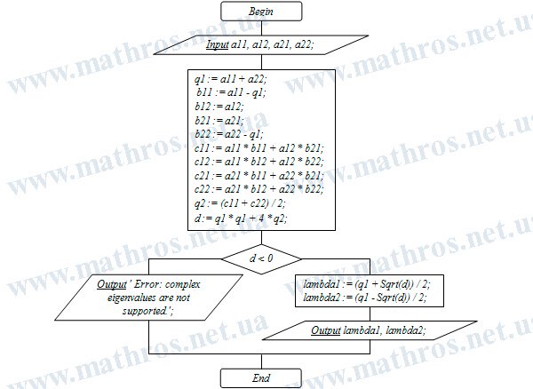
If you are interested not only in calculating by hand but also in turning a mathematical method into working code, the flowchart below will be a good basis for practice. It shows the logic of a program that finds the eigenvalues of a second-order matrix using the Faddeev method.
Try to implement this algorithm in Pascal, Python, C++, JavaScript, or any other language you are comfortable working with. This way, you will better see how formulas from theory turn into variables, calculations, conditions, and the final result.