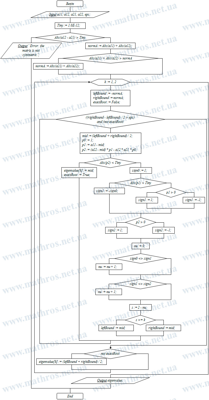
The eigenvalues of a symmetric tridiagonal matrix can be found without expanding the characteristic determinant or directly solving a high-degree algebraic equation. The bisection method is used for this purpose and is based on the properties of a Sturm sequence. First, we construct a sequence of polynomials. Next, we use the sign changes in this sequence to determine where the required eigenvalue is located. Finally, we gradually narrow the interval containing that eigenvalue.
Eigenvalues of a Symmetric Tridiagonal Matrix: Problem Statement
Consider a symmetric tridiagonal matrix \( A \) of order \( n \):
\[
A=
\begin{pmatrix}
a_1 & b_1 & 0 & \cdots & 0 & 0\\
b_1 & a_2 & b_2 & \cdots & 0 & 0\\
0 & b_2 & a_3 & \ddots & 0 & 0\\
\vdots & \vdots & \ddots & \ddots & b_{n-2} & 0\\
0 & 0 & 0 & b_{n-2} & a_{n-1} & b_{n-1}\\
0 & 0 & 0 & 0 & b_{n-1} & a_n
\end{pmatrix}.
\]
The elements of the matrix \( A \) can be defined in general form as follows:
\[
a_{ij}=
\begin{cases}
a_i, & i=j,\\[4pt]
b_i, & j=i+1,\\[4pt]
b_j, & i=j+1,\\[4pt]
0, & |i-j|>1.
\end{cases}
\]
The nonzero elements of such a matrix appear only on the main diagonal and the two diagonals directly next to it. The symmetry of the matrix means that
\[
a_{ij}=a_{ji}.
\]
Therefore, each element \( b_i \) above the main diagonal is equal to the corresponding element below it.
Symmetric tridiagonal matrices appear in many practical problems involving numerical methods. In addition, finding the eigenvalues of an arbitrary symmetric matrix is often reduced to a similar problem for a symmetric tridiagonal matrix. Because of its special structure, the amount of computation required is significantly reduced.
From this point on, we assume that all off-diagonal elements \( b_i \) are nonzero:
\[
b_i\neq 0,
\qquad
i=1,2,\dots,n-1.
\]
Under this condition, the matrix is irreducible, and all its eigenvalues are real and pairwise distinct. Let us arrange them in descending order:
\[
\lambda_1>\lambda_2>\dots>\lambda_n.
\]
If some element \( b_i \) is equal to zero, the matrix splits into separate symmetric tridiagonal blocks. In that case, the eigenvalues can be found separately for each block.
Sturm Sequence: Constructing Leading Principal Minors
To construct the Sturm sequence, consider the leading principal submatrices of the matrix \( A \). Let \( A_i \) denote the leading principal submatrix of order \( i \):
\[
A_i=
\begin{pmatrix}
a_1 & b_1 & 0 & \cdots & 0\\
b_1 & a_2 & b_2 & \cdots & 0\\
0 & b_2 & a_3 & \ddots & \vdots\\
\vdots & \vdots & \ddots & \ddots & b_{i-1}\\
0 & 0 & \cdots & b_{i-1} & a_i
\end{pmatrix},
\qquad
i=1,2,\dots,n.
\]
For each submatrix \( A_i \), define the polynomial
\[
p_i(\lambda)
=
\det\left(A_i-\lambda\cdot I_i\right),
\qquad
i=1,2,\dots,n,
\]
where \( I_i \) is the identity matrix of order \( i \). We also set
\[
p_0(\lambda)=1.
\]
For the leading principal submatrix of order \( 1 \), we have
\[
p_1(\lambda)=a_1-\lambda.
\]
Now consider the leading principal submatrix of order \( 2 \). For this matrix, we obtain
\[
p_2(\lambda)
=
\det
\begin{pmatrix}
a_1-\lambda & b_1\\
b_1 & a_2-\lambda
\end{pmatrix}
=
(a_1-\lambda)\cdot(a_2-\lambda)-b_1^2.
\]
Since
\[
p_0(\lambda)=1,
\qquad
p_1(\lambda)=a_1-\lambda,
\]
the last equality can be written as
\[
p_2(\lambda)
=
(a_2-\lambda)\cdot p_1(\lambda)-b_1^2\cdot p_0(\lambda).
\]
In the same way, for leading principal submatrices of higher orders, we obtain the recurrence relation
\[
p_i(\lambda)
=
(a_i-\lambda)\cdot p_{i-1}(\lambda)-b_{i-1}^{2}\cdot p_{i-2}(\lambda),
\qquad
i=2,3,\dots,n.
\]
Thus, the following polynomials are computed one after another:
\[
p_0(\lambda),
p_1(\lambda),
p_2(\lambda),\dots,
p_n(\lambda).
\]
Since \( A_n=A \), the last polynomial in this sequence is the characteristic polynomial of the matrix:
\[
p_n(\lambda)
=
\det\left(A-\lambda\cdot I\right).
\]
Therefore, the eigenvalues of the matrix are the roots of the equation
\[
p_n(\lambda)=0.
\]
The polynomials \( p_0(\lambda),p_1(\lambda),p_2(\lambda),\dots,p_n(\lambda) \) form a Sturm sequence. There is no need to expand each determinant separately to compute them. It is enough to apply the recurrence relation step by step, using only the two previous values.
Property of the Sturm Sequence: Counting Eigenvalues
Let \( \mu \) be a given number. Substitute it for the parameter \( \lambda \) and compute the numerical sequence
\[
p_0(\mu),
p_1(\mu),
p_2(\mu),\dots,
p_n(\mu).
\]
Let \( \nu(\mu) \) denote the number of sign changes between consecutive nonzero terms of this sequence. The key property of the Sturm sequence is that \( \nu(\mu) \) equals the number of eigenvalues of the matrix that are strictly less than \( \mu \).
If \( \mu \) is not an eigenvalue of the matrix, the number of eigenvalues strictly greater than \( \mu \) is given by
\[
s(\mu)=n-\nu(\mu).
\]
Therefore, the value \( s(\mu) \) shows how many eigenvalues satisfy the inequality
\[
\lambda_i>\mu.
\]
This property allows us to determine the position of the \( k \)-th eigenvalue without computing it directly. If \( s(\mu)\geq k \), then at least \( k \) eigenvalues lie to the right of \( \mu \). Therefore, for the \( k \)-th eigenvalue arranged in descending order, we have
\[
\lambda_k>\mu.
\]
If \( s(\mu)<k \), then fewer than \( k \) eigenvalues lie to the right of \( \mu \). In this case,
\[
\lambda_k\leq\mu.
\]
When counting sign changes, an intermediate value \( p_i(\mu) \) may be equal to zero. In that case, we assign it a sign opposite to that of the preceding term \( p_{i-1}(\mu) \). This rule is used only to determine the number of sign changes correctly and does not change the actual value of the polynomial.
Provided that \( b_i\neq 0 \), two consecutive terms of the Sturm sequence cannot both be zero.
If \( p_n(\mu)=0 \), then \( \mu \) is an exact eigenvalue of the matrix.
Bisection Method: Computational Procedure
To apply the bisection method, we first need to determine an interval containing all the eigenvalues of the matrix. If the bounds of this interval are not known in advance, we can use the infinity norm of the matrix:
\[
\lVert A\rVert_{\infty}
=
\max_{1\leq i\leq n}
\left(
|b_{i-1}|+|a_i|+|b_i|
\right),
\qquad
b_0=b_n=0.
\]
All eigenvalues of the symmetric matrix \( A \) lie within the interval
\[
-\lVert A\rVert_{\infty}
\leq
\lambda_i
\leq
\lVert A\rVert_{\infty}.
\]
Therefore, the initial endpoints can be chosen as follows:
\[
\alpha_0=-\lVert A\rVert_{\infty},
\qquad
\beta_0=\lVert A\rVert_{\infty}.
\]
To find the \( k \)-th eigenvalue, where \( k=1,2,\dots,n \), we compute the midpoint of the current interval at the \( r \)-th iteration:
\[
c_r=
\frac{\alpha_{r-1}+\beta_{r-1}}{2},
\qquad
r=1,2,3,\dots.
\]
At the point \( c_r \), we use the recurrence relation to compute the values
\[
p_0(c_r),
p_1(c_r),
p_2(c_r),\dots,
p_n(c_r).
\]
Next, we determine the number of sign changes \( \nu(c_r) \).
If \( p_n(c_r)=0 \), then \( c_r \) is an exact eigenvalue of the matrix, and the iteration can be stopped.
Otherwise, we compute the number of eigenvalues greater than \( c_r \):
\[
s(c_r)=n-\nu(c_r).
\]
If \( s(c_r)\geq k \), then
\[
\lambda_k>c_r.
\]
Therefore, the eigenvalue being sought lies in the right half of the current interval. The new endpoints are defined as
\[
\alpha_r=c_r,
\qquad
\beta_r=\beta_{r-1}.
\]
If \( s(c_r)<k \), then
\[
\lambda_k\leq c_r.
\]
In this case, the eigenvalue being sought lies in the left half of the current interval, so we set
\[
\alpha_r=\alpha_{r-1},
\qquad
\beta_r=c_r.
\]
After each iteration, the following inclusion remains valid:
\[
\lambda_k\in[\alpha_r,\beta_r],
\]
while the length of the interval is reduced by half.
The iterative process continues until the condition
\[
\frac{\beta_r-\alpha_r}{2}\leq\varepsilon,
\]
is satisfied, where \( \varepsilon \) is the desired accuracy.
After the iterations are complete, the approximate value of the \( k \)-th eigenvalue is taken as the midpoint of the final interval:
\[
\lambda_k
\approx
\frac{\alpha_r+\beta_r}{2}.
\]
The error of the obtained approximation does not exceed half the length of this interval:
\[
\left|
\lambda_k-
\frac{\alpha_r+\beta_r}{2}
\right|
\leq
\frac{\beta_r-\alpha_r}{2}.
\]
Thus, after the iterations are complete, we obtain an approximate value of \( \lambda_k \) whose absolute error does not exceed half the length of the final interval.
Eigenvalues of a Symmetric Tridiagonal Matrix: Bisection Method in Practice
Let us see how the bisection method is applied to symmetric tridiagonal matrices of different orders. In each example, we will find one specified eigenvalue by using the Sturm sequence to select the required half of the current interval.
Example 1. Find the largest eigenvalue of a symmetric tridiagonal matrix
\[
A=
\begin{pmatrix}
2 & 0.5\\
0.5 & 1
\end{pmatrix}
\]
using the bisection method with \( \varepsilon=0.1 \)
The matrix has two eigenvalues. Let us arrange them in descending order:
\[
\lambda_1>\lambda_2.
\]
We need to find the largest eigenvalue \( \lambda_1 \).
First, compute the infinity norm of the matrix:
\[
\lVert A\rVert_{\infty}
=
\max
\left\{
|2|+|0.5|,
|0.5|+|1|
\right\}
=
\max\left\{2.5,1.5\right\}
=
2.5.
\]
Therefore, all eigenvalues of the matrix lie within the interval
\[
[\alpha_0,\beta_0]=[-2.5,2.5].
\]
Construct the Sturm sequence:
\[
\begin{gathered}
p_0(\mu)=1,\\[4pt]
p_1(\mu)=2-\mu,\\[4pt]
p_2(\mu)=(1-\mu)\cdot p_1(\mu)-0.5^2\cdot p_0(\mu).
\end{gathered}
\]
At the first iteration, compute the midpoint of the initial interval:
\[
c_1=
\frac{-2.5+2.5}{2}=0.
\]
Now compute the terms of the Sturm sequence:
\[
\begin{gathered}
p_0(0)=1,\\[4pt]
p_1(0)=2-0=2,\\[4pt]
p_2(0)=(1-0)\cdot 2-0.5^2\cdot 1=1\cdot 2-0.25\cdot 1=1.75.
\end{gathered}
\]
We obtain the following sequence of signs:
\[
+,\ +,\ +.
\]
The number of sign changes is \( \nu(0)=0 \). Therefore, the number of eigenvalues greater than \( 0 \) is
\[
s(0)=2-\nu(0)=2-0=2.
\]
Since \( s(0)\geq 1 \), the largest eigenvalue lies in the right half of the initial interval:
\[
\lambda_1\in[0,2.5].
\]
The remaining iterations are performed in the same way:
| \( r \) | \( c_r \) | \( \bigl(p_0(c_r),p_1(c_r),p_2(c_r)\bigr) \) | \( \nu(c_r) \) | \( s(c_r) \) | New interval |
|---|---|---|---|---|---|
| 1 | \( 0 \) | \( (1, 2, 1.75) \) | 0 | 2 | \( [0,2.5] \) |
| 2 | \( 1.25 \) | \( (1, 0.75, -0.438) \) | 1 | 1 | \( [1.25,2.5] \) |
| 3 | \( 1.875 \) | \( (1, 0.125, -0.359) \) | 1 | 1 | \( [1.875,2.5] \) |
| 4 | \( 2.188 \) | \( (1, -0.188, -0.027) \) | 1 | 1 | \( [2.188,2.5] \) |
| 5 | \( 2.344 \) | \( (1, -0.344, 0.212) \) | 2 | 0 | \( [2.188,2.344] \) |
After the fifth iteration, the eigenvalue being sought lies within the interval
\[
\lambda_1\in[2.188,2.344].
\]
Check the stopping condition:
\[
\frac{\beta_5-\alpha_5}{2}
\approx
\frac{2.344-2.188}{2}
=
0.078.
\]
Since
\[
0.078\leq 0.1,
\]
we stop the iterative process.
We take the midpoint of the final interval as the approximate value of \( \lambda_1 \):
\[
\lambda_1
\approx
\frac{2.188+2.344}{2}
=
2.266.
\]
Therefore, the largest eigenvalue of the matrix is approximately
\[
\lambda_1\approx 2.266.
\]
Example 2. Find the second-largest eigenvalue of a symmetric tridiagonal matrix
\[
A=
\begin{pmatrix}
3 & 1 & 0\\
1 & 2 & 1\\
0 & 1 & 0
\end{pmatrix}
\]
using the bisection method with \( \varepsilon=0.1 \)
The matrix has three eigenvalues. Let us arrange them in descending order:
\[
\lambda_1>\lambda_2>\lambda_3.
\]
We need to find the second-largest eigenvalue \( \lambda_2 \).
Compute the infinity norm of the matrix:
\[
\lVert A\rVert_{\infty}
=
\max
\left\{
|3|+|1|,
|1|+|2|+|1|,
|1|+|0|
\right\}
=
\max\left\{4,4,1\right\}=4.
\]
Therefore, the initial interval is
\[
[\alpha_0,\beta_0]=[-4,4].
\]
For the given matrix, the Sturm sequence is defined by the formulas
\[
\begin{gathered}
p_0(\mu)=1,\\[4pt]
p_1(\mu)=3-\mu,\\[4pt]
p_2(\mu)=(2-\mu)\cdot p_1(\mu)-p_0(\mu),\\[4pt]
p_3(\mu)=(-\mu)\cdot p_2(\mu)-p_1(\mu).
\end{gathered}
\]
At the first iteration, the midpoint of the initial interval is
\[
c_1=
\frac{-4+4}{2}=0.
\]
Compute the terms of the Sturm sequence:
\[
\begin{gathered}
p_0(0)=1,\\[4pt]
p_1(0)=3-0=3,\\[4pt]
p_2(0)=(2-0)\cdot 3-1=5,\\[4pt]
p_3(0)=(-0)\cdot 5-3=-3.
\end{gathered}
\]
The sequence of signs is
\[
+,\ +,\ +,\ -.
\]
The number of sign changes is \( \nu(0)=1 \). Therefore, the number of eigenvalues greater than \( 0 \) is
\[
s(0)=3-\nu(0)=3-1=2.
\]
Since \( s(0)\geq 2 \), the second-largest eigenvalue lies in the right half of the initial interval:
\[
\lambda_2\in[0,4].
\]
The remaining calculations are shown in the table:
| \( r \) | \( c_r \) | \( \bigl(p_0(c_r),p_1(c_r),p_2(c_r),p_3(c_r)\bigr) \) | \( \nu(c_r) \) | \( s(c_r) \) | New interval |
|---|---|---|---|---|---|
| 1 | \( 0 \) | \( (1, 3, 5, -3) \) | 1 | 2 | \( [0,4] \) |
| 2 | \( 2 \) | \( (1, 1, -1, 1) \) | 2 | 1 | \( [0,2] \) |
| 3 | \( 1 \) | \( (1, 2, 1, -3) \) | 1 | 2 | \( [1,2] \) |
| 4 | \( 1.5 \) | \( (1, 1.5, -0.25, -1.125) \) | 1 | 2 | \( [1.5,2] \) |
| 5 | \( 1.75 \) | \( (1, 1.25, -0.688, -0.047) \) | 1 | 2 | \( [1.75,2] \) |
| 6 | \( 1.875 \) | \( (1, 1.125, -0.859, 0.486) \) | 2 | 1 | \( [1.75,1.875] \) |
After the sixth iteration, we have
\[
\lambda_2\in[1.75,1.875].
\]
Check the stopping condition:
\[
\frac{\beta_6-\alpha_6}{2}
\approx
\frac{1.875-1.75}{2}
=
0.063.
\]
Since
\[
0.063\leq 0.1,
\]
we stop the iterative process.
The approximate value of the second-largest eigenvalue is
\[
\lambda_2
\approx
\frac{1.75+1.875}{2}
=
1.813.
\]
Therefore, the second-largest eigenvalue of the matrix is approximately
\[
\lambda_2\approx 1.813.
\]
Example 3. Find the third-largest eigenvalue of a symmetric tridiagonal matrix
\[
A=
\begin{pmatrix}
6 & 1 & 0 & 0\\
1 & 4 & 1 & 0\\
0 & 1 & 2 & 1\\
0 & 0 & 1 & 1
\end{pmatrix}
\]
using the bisection method with \( \varepsilon=0.1 \)
The matrix has four eigenvalues. Let us arrange them in descending order:
\[
\lambda_1>\lambda_2>\lambda_3>\lambda_4.
\]
We need to find the third-largest eigenvalue \( \lambda_3 \).
Compute the infinity norm of the matrix:
\[
\lVert A\rVert_{\infty}
=
\max
\left\{
|6|+|1|,
|1|+|4|+|1|,
|1|+|2|+|1|,
|1|+|1|
\right\}
=
\max\left\{7,6,4,2\right\}
=7.
\]
Therefore, all eigenvalues of the matrix lie within the interval
\[
[\alpha_0,\beta_0]=[-7,7].
\]
Construct the Sturm sequence:
\[
\begin{gathered}
p_0(\mu)=1,\\[4pt]
p_1(\mu)=6-\mu,\\[4pt]
p_2(\mu)=(4-\mu)\cdot p_1(\mu)-p_0(\mu),\\[4pt]
p_3(\mu)=(2-\mu)\cdot p_2(\mu)-p_1(\mu),\\[4pt]
p_4(\mu)=(1-\mu)\cdot p_3(\mu)-p_2(\mu).
\end{gathered}
\]
At the first iteration, the midpoint of the initial interval is
\[
c_1=
\frac{-7+7}{2}=0.
\]
Compute the terms of the Sturm sequence:
\[
\begin{gathered}
p_0(0)=1,\\[4pt]
p_1(0)=6-0=6,\\[4pt]
p_2(0)=(4-0)\cdot 6-1=23,\\[4pt]
p_3(0)=(2-0)\cdot 23-6=40,\\[4pt]
p_4(0)=(1-0)\cdot 40-23=17.
\end{gathered}
\]
We obtain the following sequence of signs:
\[
+,\ +,\ +,\ +,\ +.
\]
The number of sign changes is \( \nu(0)=0 \). Therefore, the number of eigenvalues greater than \( 0 \) is
\[
s(0)=4-\nu(0)=4-0=4.
\]
Since \( s(0)\geq 3 \), the third-largest eigenvalue lies in the right half of the initial interval:
\[
\lambda_3\in[0,7].
\]
The remaining iterations are shown in the table:
| \( r \) | \( c_r \) | \( \bigl(p_0(c_r),p_1(c_r),p_2(c_r),p_3(c_r),p_4(c_r)\bigr) \) | \( \nu(c_r) \) | \( s(c_r) \) | New interval |
|---|---|---|---|---|---|
| 1 | \( 0 \) | \( (1, 6, 23, 40, 17) \) | 0 | 4 | \( [0,7] \) |
| 2 | \( 3.5 \) | \( (1, 2.5, 0.25, -2.875, 6.938) \) | 2 | 2 | \( [0,3.5] \) |
| 3 | \( 1.75 \) | \( (1, 4.25, 8.563, -2.109, -6.98) \) | 1 | 3 | \( [1.75,3.5] \) |
| 4 | \( 2.625 \) | \( (1, 3.375, 3.641, -5.65, 5.541) \) | 2 | 2 | \( [1.75,2.625] \) |
| 5 | \( 2.188 \) | \( (1, 3.813, 5.91, -4.921, -0.067) \) | 1 | 3 | \( [2.188,2.625] \) |
| 6 | \( 2.406 \) | \( (1, 3.594, 4.728, -5.514, 3.027) \) | 2 | 2 | \( [2.188,2.406] \) |
| 7 | \( 2.297 \) | \( (1, 3.703, 5.307, -5.279, 1.539) \) | 2 | 2 | \( [2.188,2.297] \) |
After the seventh iteration, we obtain the interval
\[
\lambda_3\in[2.188,2.297].
\]
Check the stopping condition:
\[
\frac{\beta_7-\alpha_7}{2}
\approx
\frac{2.297-2.188}{2}
=
0.055.
\]
Since
\[
0.055\leq 0.1,
\]
we stop the iterative process.
We take the midpoint of the final interval as the approximate value of the third-largest eigenvalue:
\[
\lambda_3
\approx
\frac{2.188+2.297}{2}
=
2.242.
\]
Therefore, the third-largest eigenvalue of the matrix is approximately
\[
\lambda_3\approx 2.242.
\]
What to Read Next: Other Ways to Compute Eigenvalues
The bisection method is only one way to study the spectrum of a matrix. Next, you can explore other algorithms and compare which types of problems are easier to solve with each method.
- Jacobi Rotation Method: Eigenvalues of a Symmetric Matrix — Learn how successive rotations eliminate off-diagonal elements and help compute all the eigenvalues of a symmetric matrix.
- Power Method: Dominant Eigenvalue — See how repeated multiplication of a matrix by a vector can be used to approximate the eigenvalue with the largest absolute value and its corresponding eigenvector.
- Deflation Method: Second Eigenvalue of a Matrix — Learn how to modify a matrix after finding the first eigenvalue and then compute the next one.
Algorithm Implementation: Computing Eigenvalues of a Symmetric Tridiagonal Matrix in Code
If you enjoy programming, this is a great time to move from theory to your own implementation. The flowchart already contains all the steps required for the computation, so you can implement the algorithm in Pascal, Python, C++, JavaScript, or any other programming language you are comfortable with.
This is a useful opportunity not only to strengthen your understanding of the bisection method but also to see how a mathematical algorithm becomes a complete program. Such a program can compute the eigenvalues of a symmetric tridiagonal matrix and help you better understand the connection between numerical methods and practical programming.