When studying the eigenvalues of a symmetric matrix, the rotation method is useful because it allows us to find them without forming the characteristic equation. The idea of the method is quite simple: step by step, we transform the original matrix so that it becomes closer and closer to a diagonal matrix.
As a result, the diagonal elements of the obtained matrix can be taken as approximate eigenvalues. In addition, this method also allows us to find the corresponding eigenvectors, which makes it convenient for solving the complete eigenvalue problem.
Eigenvalues of a Symmetric Matrix: When the Method Applies and What Its Main Idea Is
Let us start with the main point. In this form, the rotation method is applied to real symmetric matrices. That is, to matrices \( A \) for which the following condition holds:
\[
A=A^T.
\]
In other words, the elements of the matrix are placed symmetrically with respect to the main diagonal:
\[
a_{ij}=a_{ji},\qquad i,j=1,2,\dots,n.
\]
Why is this condition so important? Because for symmetric matrices, orthogonal rotations work especially well. After such transformations, the matrix remains symmetric, and its eigenvalues do not change.
This method is also often called the Jacobi rotation method. In a numerical methods course, this name appears very often, so it is worth remembering.
Suppose we are given the matrix
\[
A=
\begin{pmatrix}
a_{11} & a_{12} & \dots & a_{1n}\\
a_{21} & a_{22} & \dots & a_{2n}\\
\vdots & \vdots & \ddots & \vdots\\
a_{n1} & a_{n2} & \dots & a_{nn}
\end{pmatrix},
\qquad A=A^T.
\]
We need to find its eigenvalues
\[
\lambda_1,\lambda_2,\dots,\lambda_n.
\]
But the rotation method allows us to do a little more. It finds not only the eigenvalues but also the corresponding eigenvectors. That is why we say that the method makes it possible to solve the complete eigenvalue problem.
Of course, we could form the characteristic equation. But is this always convenient? No. For matrices of large order, the characteristic polynomial can become bulky, and its roots are not always easy to find.
So the rotation method works differently. The original matrix is gradually transformed into a diagonal or almost diagonal matrix. For nonsymmetric matrices, this approach is usually not used without additional changes, because its main advantage appears exactly due to the symmetry of the matrix.
Therefore, the goal of the method is this: instead of finding the roots of a complicated characteristic equation, we gradually reduce the off-diagonal elements of the matrix. When they become small enough, the eigenvalues can be read off from the main diagonal.
Similarity Transformation: Why Eigenvalues Are Preserved
Now let us move on to the foundation of the method. How can we change a matrix without changing its eigenvalues? For this purpose, we use a similarity transformation.
Suppose the matrix \( A \) is transformed into the matrix \( \Lambda \) by the formula
\[
\Lambda=U^{-1}\cdot A\cdot U,
\]
where \( U \) is a nonsingular matrix.
Matrices \( A \) and \( \Lambda \), connected by such a transformation, have the same eigenvalues. In other words, the form of the matrix changes, but its spectrum is preserved.
In the rotation method, the matrix \( U \) is chosen to be orthogonal. For an orthogonal matrix, we have
\[
U^{-1}=U^T.
\]
Therefore, the similarity transformation can be written as
\[
\Lambda=U^T\cdot A\cdot U.
\]
This is convenient from a computational point of view. After all, instead of finding the inverse matrix, it is enough to take the transpose.
The rotation method does not try to immediately find a single matrix \( U \) that will make the matrix \( A \) diagonal. This is usually difficult. That is why the process is built step by step.
Let us denote the initial matrix as
\[
A^{(0)}=A.
\]
Next, we construct a sequence of matrices
\[
A^{(0)}, A^{(1)}, A^{(2)},\dots,A^{(k)}.
\]
Each next matrix is obtained from the previous one using an orthogonal similarity transformation. Therefore, all these matrices have the same eigenvalues.
In the end, we need to obtain a matrix that is close to diagonal:
\[
A^{(k)}\approx
\begin{pmatrix}
\lambda_1 & 0 & \dots & 0\\
0 & \lambda_2 & \dots & 0\\
\vdots & \vdots & \ddots & \vdots\\
0 & 0 & \dots & \lambda_n
\end{pmatrix}.
\]
This is exactly why the method works in a logical way. We do not change the eigenvalues, but we gradually change the form of the matrix. As a result, it becomes a matrix from which these values are easy to read off.
Rotation Matrix: How One Step of the Method Is Performed
Now we need to understand which matrix is used to perform one step of the method. At each iteration, a special orthogonal rotation matrix is used. It is denoted as
\[
U_{i_kj_k}(\phi_k).
\]
Here \( k \) is the iteration number, \( i_k \) and \( j_k \) are the indices of the selected off-diagonal element, and \( \phi_k \) is the rotation angle.
The matrix \( U_{i_kj_k}(\phi_k) \) is almost the same as the identity matrix. It differs from it only in four elements:
\[
\begin{gathered}
u_{i_ki_k}=\cos(\phi_k),
\qquad
u_{i_kj_k}=-\sin(\phi_k),[4pt]
u_{j_ki_k}=\sin(\phi_k),
\qquad
u_{j_kj_k}=\cos(\phi_k).
\end{gathered}
\]
All other diagonal elements are equal to one, and all remaining off-diagonal elements are equal to zero.
For convenience, let us introduce the notation
\[
c_k=\cos(\phi_k),
\qquad
s_k=\sin(\phi_k).
\]
Then the rotation matrix can be shown schematically as
\[
U_{i_kj_k}(\phi_k)=
\begin{pmatrix}
1 & \dots & 0 & \dots & 0 & \dots & 0\\
\vdots & \ddots & \vdots & & \vdots & & \vdots\\
0 & \dots & c_k & \dots & -s_k & \dots & 0\\
\vdots & & \vdots & \ddots & \vdots & & \vdots\\
0 & \dots & s_k & \dots & c_k & \dots & 0\\
\vdots & & \vdots & & \vdots & \ddots & \vdots\\
0 & \dots & 0 & \dots & 0 & \dots & 1
\end{pmatrix}.
\]
What does such a matrix do? It changes only two rows and two columns associated with the indices \( i_k \) and \( j_k \). The rest of the matrix structure remains unchanged.
At the \( k \)-th step of the method, the following transformation is performed:
\[
A^{(k)}
=
U_{i_kj_k}^{T}(\phi_k)\cdot
A^{(k-1)}\cdot
U_{i_kj_k}(\phi_k),
\qquad k=1,2,3,\dots.
\]
From the previous section, it is already clear why such a transformation does not change the eigenvalues. Now another point is important: this transformation makes it possible to gradually reduce the off-diagonal elements.
If we need to perform one step of the method in detail or implement it in a program, it is convenient to split the transformation into two actions. First, we introduce an auxiliary matrix \( B \):
\[
B=A^{(k-1)}\cdot U_{i_kj_k}(\phi_k).
\]
Then we find the new matrix
\[
A^{(k)}=U_{i_kj_k}^{T}(\phi_k)\cdot B.
\]
That is, the full transformation
\[
A^{(k)}
=
U_{i_kj_k}^{T}(\phi_k)\cdot
A^{(k-1)}\cdot
U_{i_kj_k}(\phi_k)
\]
can be performed as two consecutive multiplications. First, we multiply the current matrix on the right by the rotation matrix, and then we multiply the result on the left by the transposed rotation matrix.
During the first multiplication, only the \( i_k \)-th and \( j_k \)-th columns change. For them, we have
\[
\begin{gathered}
b_{zi_k}
=
a_{zi_k}^{(k-1)}\cdot c_k
+
a_{zj_k}^{(k-1)}\cdot s_k,
\qquad z=1,2,\dots,n,\\[4pt]
b_{zj_k}
=
-a_{zi_k}^{(k-1)}\cdot s_k
+
a_{zj_k}^{(k-1)}\cdot c_k,
\qquad z=1,2,\dots,n.
\end{gathered}
\]
Next, during the second multiplication, only the \( i_k \)-th and \( j_k \)-th rows change. For them, we obtain
\[
\begin{gathered}
a_{i_kz}^{(k)}
=
b_{i_kz}\cdot c_k
+
b_{j_kz}\cdot s_k,
\qquad z=1,2,\dots,n,\\[4pt]
a_{j_kz}^{(k)}
=
-b_{i_kz}\cdot s_k
+
b_{j_kz}\cdot c_k,
\qquad z=1,2,\dots,n.
\end{gathered}
\]
So, one step of the method has a clear structure. First, we multiply on the right, which changes two columns. Then we multiply on the left, which changes two rows. As a result, exactly those elements associated with the selected indices are changed.
But now the next question appears: how do we choose the indices \( i_k \), \( j_k \), and the angle \( \phi_k \) itself? This is exactly what determines which element will be made zero at the current step.
Eigenvalues of a Symmetric Matrix: Choosing the Element and the Rotation Angle
At each step, we need to choose the off-diagonal element that we will make zero. Since the matrix is symmetric, it is enough to consider the elements located, for example, above the main diagonal.
Most often, we choose the off-diagonal element of the matrix \( A^{(k-1)} \) with the largest absolute value. That is, the indices \( i_k \) and \( j_k \) are determined from the condition
\[
\left|a_{i_kj_k}^{(k-1)}\right|
=
\max_{1\leq i<j\leq n}
\left|a_{ij}^{(k-1)}\right|.
\]
Why do we choose the largest element? Because this way, at each step, the off-diagonal part of the matrix is reduced most actively. And this is exactly the part we want to gradually remove.
After choosing the indices \( i_k \) and \( j_k \), we need to find the angle \( \phi_k \). It is chosen so that after the transformation, the selected element becomes zero:
\[
a_{i_kj_k}^{(k)}=0.
\]
Now let us write the formula for this element after the rotation. Taking into account the symmetry of the matrix \( A^{(k-1)} \), we have
\[
a_{i_kj_k}^{(k)}
=
a_{i_kj_k}^{(k-1)}\cdot \cos(2\cdot\phi_k)
+
\frac{
a_{j_kj_k}^{(k-1)}-a_{i_ki_k}^{(k-1)}
}{2}
\cdot \sin(2\cdot\phi_k).
\]
According to the method, this element must be equal to zero. Therefore, we obtain the equation
\[
a_{i_kj_k}^{(k-1)}\cdot \cos(2\cdot\phi_k)
+
\frac{
a_{j_kj_k}^{(k-1)}-a_{i_ki_k}^{(k-1)}
}{2}
\cdot \sin(2\cdot\phi_k)
=
0.
\]
From this, it follows that
\[
\tan(2\cdot\phi_k)
=
\frac{
2\cdot a_{i_kj_k}^{(k-1)}
}{
a_{i_ki_k}^{(k-1)}-a_{j_kj_k}^{(k-1)}
}.
\]
So, if
\[
a_{i_ki_k}^{(k-1)}\neq a_{j_kj_k}^{(k-1)},
\]
then the rotation angle can be found by the formula
\[
\phi_k
=
\frac{1}{2}\cdot
\arctan\left(
\frac{
2\cdot a_{i_kj_k}^{(k-1)}
}{
a_{i_ki_k}^{(k-1)}-a_{j_kj_k}^{(k-1)}
}
\right).
\]
If
\[
a_{i_ki_k}^{(k-1)}=a_{j_kj_k}^{(k-1)},
\]
then we take
\[
\phi_k=\frac{\pi}{4}.
\]
Together, this can be written as
\[
\phi_k=
\begin{cases}
\dfrac{1}{2}\cdot \arctan\left(
\dfrac{
2\cdot a_{i_kj_k}^{(k-1)}
}{
a_{i_ki_k}^{(k-1)}-a_{j_kj_k}^{(k-1)}
}
\right),
& a_{i_ki_k}^{(k-1)}\neq a_{j_kj_k}^{(k-1)}, \\[12pt]
\dfrac{\pi}{4},
& a_{i_ki_k}^{(k-1)}=a_{j_kj_k}^{(k-1)}.
\end{cases}
\]
So, the logic of the iteration is clear. First, we choose the largest off-diagonal element. Then we find the rotation angle. After that, we perform the transformation, and this element becomes zero.
Of course, after one step, the whole matrix will not become diagonal yet. Also, some other off-diagonal elements may change. But in general, after many such rotations, the off-diagonal part of the matrix becomes smaller and smaller.
This is why the rotation method is iterative. It gradually brings the matrix closer to a form from which the eigenvalues are easy to obtain.
Completion of the Method: Eigenvalues and Eigenvectors
Now we only need to understand when to stop the iterative process. Since the rotation method is approximate, the accuracy \( \varepsilon \) is chosen in advance.
The iterations continue until the sum of the squares of the off-diagonal elements of the matrix \( A^{(k)} \) becomes less than or equal to the given accuracy:
\[
\sum_{\substack{i,j=1\ i\neq j}}^{n}
\left(a_{ij}^{(k)}\right)^2
\leq
\varepsilon.
\]
This condition means that the off-diagonal elements are already small enough. In other words, the matrix \( A^{(k)} \) has become close to diagonal.
After that, the approximate eigenvalues of the original matrix \( A \) are taken from the diagonal of the matrix \( A^{(k)} \):
\[
\lambda_1\approx a_{11}^{(k)},
\qquad
\lambda_2\approx a_{22}^{(k)},
\qquad
\lambda_3\approx a_{33}^{(k)},
\qquad
\dots,
\qquad
\lambda_n\approx a_{nn}^{(k)}.
\]
Here it is important to remember one detail. These values are not necessarily arranged in increasing or decreasing order. Their order depends on how the iterations proceed.
This is how we find the eigenvalues of a symmetric matrix using the rotation method. We do not form the characteristic equation. Instead, we gradually reduce the off-diagonal elements and obtain approximate eigenvalues from the diagonal.
Now let us return to eigenvectors. At each step, we use a certain rotation matrix:
\[
U_{i_1j_1}(\phi_1),
\qquad
U_{i_2j_2}(\phi_2),
\qquad
\dots,
\qquad
U_{i_kj_k}(\phi_k).
\]
If we multiply all these matrices, we obtain the matrix
\[
Q^{(k)}
=
U_{i_1j_1}(\phi_1)\cdot
U_{i_2j_2}(\phi_2)\cdot
\dots
\cdot
U_{i_kj_k}(\phi_k).
\]
This matrix accumulates all the rotations that have been performed. Therefore, it connects the original matrix \( A \) with the approximately diagonal matrix \( A^{(k)} \):
\[
A^{(k)}
\approx
\left(Q^{(k)}\right)^T\cdot A\cdot Q^{(k)}.
\]
The columns of the matrix \( Q^{(k)} \) are approximate eigenvectors of the original matrix \( A \). Each such column corresponds to a certain eigenvalue located on the diagonal of the matrix \( A^{(k)} \).
So, the rotation method allows us to find not only eigenvalues but also eigenvectors. This is one of the main reasons why it is useful for the complete eigenvalue problem of a symmetric matrix.
Let us summarize the general scheme. First, we check whether the given matrix is symmetric. Next, we choose the off-diagonal element with the largest absolute value. Then we find the rotation angle and make this element zero. After that, we repeat the process until the required accuracy is reached.
As a result, the diagonal elements give approximate eigenvalues, and the product of the rotation matrices gives approximate eigenvectors.
Practical Part: Examples of Calculations Using the Rotation Method
Now let us look at how the rotation method works on specific matrices. In each example, we will gradually make the largest off-diagonal elements equal to zero and check whether the matrix has become close enough to diagonal. This will help us see how approximate eigenvalues and eigenvectors are obtained from the theoretical formulas.
Example 1. Find the eigenvalues of a symmetric matrix and the corresponding eigenvectors using the rotation method with accuracy \( \varepsilon=0.1 \):
\[
A=
\begin{pmatrix}
4 & 1\\
1 & 3
\end{pmatrix}.
\]
We have a symmetric \( 2\times 2 \) matrix. Let us denote
\[
A^{(0)}=A=
\begin{pmatrix}
4 & 1\\
1 & 3
\end{pmatrix}.
\]
First, let us check the sum of the squares of the off-diagonal elements:
\[
S^{(0)}=1^2+1^2=2.
\]
Since
\[
2>0.1,
\]
we need to perform the transformation.
In a \( 2\times 2 \) matrix, there is only one off-diagonal element above the main diagonal, \( a_{12}^{(0)}=1 \). Therefore, we take \( i_1=1 \) and \( j_1=2 \). Let us find the rotation angle:
\[
\tan(2\cdot\phi_1)
=
\frac{2\cdot a_{12}^{(0)}}{a_{11}^{(0)}-a_{22}^{(0)}}
=
\frac{2\cdot 1}{4-3}
=
2.
\]
From this,
\[
\phi_1=\frac{1}{2}\cdot\arctan(2)\approx 0.5536.
\]
Then
\[
c_1=\cos(\phi_1)\approx 0.8507,
\qquad
s_1=\sin(\phi_1)\approx 0.5257.
\]
The rotation matrix has the form
\[
U_{12}(\phi_1)=
\begin{pmatrix}
0.8507 & -0.5257\\
0.5257 & 0.8507
\end{pmatrix}.
\]
Then the transposed rotation matrix is
\[
U_{12}^{T}(\phi_1)=
\begin{pmatrix}
0.8507 & 0.5257\\
-0.5257 & 0.8507
\end{pmatrix}.
\]
We perform the transformation
\[
A^{(1)}
=
U_{12}^{T}(\phi_1)\cdot A^{(0)}\cdot U_{12}(\phi_1).
\]
Substitute the found matrices:
\[
A^{(1)}
=
\begin{pmatrix}
0.8507 & 0.5257\\
-0.5257 & 0.8507
\end{pmatrix}
\cdot
\begin{pmatrix}
4 & 1\\
1 & 3
\end{pmatrix}
\cdot
\begin{pmatrix}
0.8507 & -0.5257\\
0.5257 & 0.8507
\end{pmatrix}.
\]
After multiplying, we obtain
\[
A^{(1)}
\approx
\begin{pmatrix}
4.618 & 0\\
0 & 2.382
\end{pmatrix}.
\]
Now let us again check the sum of the squares of the off-diagonal elements:
\[
S^{(1)}=0.
\]
Since
\[
0\leq 0.1,
\]
we stop the iterative process.
So, as approximate eigenvalues, we take the diagonal elements of the matrix \( A^{(1)} \):
\[
\lambda_1\approx 4.618,
\qquad
\lambda_2\approx 2.382.
\]
Now let us find the approximate eigenvectors. Since only one rotation was performed, we have
\[
Q^{(1)}=U_{12}(\phi_1).
\]
Therefore,
\[
Q^{(1)}
=
\begin{pmatrix}
0.8507 & -0.5257\\
0.5257 & 0.8507
\end{pmatrix}.
\]
The columns of this matrix are the approximate eigenvectors of the original matrix. Therefore,
\[
v_1\approx
\begin{pmatrix}
0.8507\\
0.5257
\end{pmatrix},
\qquad
v_2\approx
\begin{pmatrix}
-0.5257\\
0.8507
\end{pmatrix}.
\]
The first column corresponds to the eigenvalue \( \lambda_1\approx 4.618 \), and the second column corresponds to the eigenvalue \( \lambda_2\approx 2.382 \).
Example 2. Find the eigenvalues of a symmetric matrix and the corresponding eigenvectors using the rotation method with accuracy \( \varepsilon=0.1 \):
\[
A=
\begin{pmatrix}
4 & 1 & 1\\
1 & 3 & 0\\
1 & 0 & 2
\end{pmatrix}.
\]
Let us denote
\[
A^{(0)}=
\begin{pmatrix}
4 & 1 & 1\\
1 & 3 & 0\\
1 & 0 & 2
\end{pmatrix}.
\]
First, let us find the sum of the squares of the off-diagonal elements:
\[
S^{(0)}
=
1^2+1^2+1^2+1^2=4.
\]
Since
\[
4>0.1,
\]
we begin the iterative process.
The largest off-diagonal element by absolute value has modulus \( 1 \). We can choose, for example, \( a_{12}^{(0)}=1 \). Then \( i_1=1 \) and \( j_1=2 \). Let us find the rotation angle:
\[
\tan(2\cdot\phi_1)
=
\frac{2\cdot a_{12}^{(0)}}{a_{11}^{(0)}-a_{22}^{(0)}}
=
\frac{2\cdot 1}{4-3}
=
2.
\]
Therefore,
\[
\phi_1=\frac{1}{2}\cdot\arctan(2)\approx 0.5536.
\]
From this,
\[
c_1\approx 0.8507,
\qquad
s_1\approx 0.5257.
\]
The rotation matrix in the plane of indices \( 1 \) and \( 2 \) has the form
\[
U_{12}(\phi_1)=
\begin{pmatrix}
0.8507 & -0.5257 & 0\\
0.5257 & 0.8507 & 0\\
0 & 0 & 1
\end{pmatrix}.
\]
Then
\[
U_{12}^{T}(\phi_1)=
\begin{pmatrix}
0.8507 & 0.5257 & 0\\
-0.5257 & 0.8507 & 0\\
0 & 0 & 1
\end{pmatrix}.
\]
We perform the transformation
\[
A^{(1)}
=
U_{12}^{T}(\phi_1)\cdot A^{(0)}\cdot U_{12}(\phi_1).
\]
Substitute the matrices into this formula:
\[
A^{(1)}
=
\begin{pmatrix}
0.8507 & 0.5257 & 0\\
-0.5257 & 0.8507 & 0\\
0 & 0 & 1
\end{pmatrix}
\cdot
\begin{pmatrix}
4 & 1 & 1\\
1 & 3 & 0\\
1 & 0 & 2
\end{pmatrix}
\cdot
\begin{pmatrix}
0.8507 & -0.5257 & 0\\
0.5257 & 0.8507 & 0\\
0 & 0 & 1
\end{pmatrix}.
\]
As a result of the multiplication, we obtain
\[
A^{(1)}
\approx
\begin{pmatrix}
4.618 & 0 & 0.8507\\
0 & 2.382 & -0.5257\\
0.8507 & -0.5257 & 2
\end{pmatrix}.
\]
Now let us check the sum of the squares of the off-diagonal elements:
\[
S^{(1)}
=
2\cdot\left(0.8507^2+(-0.5257)^2\right)
\approx 2.
\]
Since
\[
2>0.1,
\]
we need to continue the calculations.
Now the largest off-diagonal element by absolute value is \( a_{13}^{(1)}\approx 0.8507 \). Therefore, we take \( i_2=1 \) and \( j_2=3 \). We calculate the angle:
\[
\tan(2\cdot\phi_2)
=
\frac{2\cdot a_{13}^{(1)}}{a_{11}^{(1)}-a_{33}^{(1)}}
=
\frac{2\cdot 0.8507}{4.618-2}
\approx 0.65.
\]
Then
\[
\phi_2\approx 0.2881,
\qquad
c_2\approx 0.9588,
\qquad
s_2\approx 0.2842.
\]
The rotation matrix in the plane of indices \( 1 \) and \( 3 \) is
\[
U_{13}(\phi_2)=
\begin{pmatrix}
0.9588 & 0 & -0.2842\\
0 & 1 & 0\\
0.2842 & 0 & 0.9588
\end{pmatrix}.
\]
Therefore,
\[
U_{13}^{T}(\phi_2)=
\begin{pmatrix}
0.9588 & 0 & 0.2842\\
0 & 1 & 0\\
-0.2842 & 0 & 0.9588
\end{pmatrix}.
\]
We perform the next transformation:
\[
A^{(2)}
=
U_{13}^{T}(\phi_2)\cdot A^{(1)}\cdot U_{13}(\phi_2).
\]
Substitute the corresponding matrices:
\[
A^{(2)}
=
\begin{pmatrix}
0.9588 & 0 & 0.2842\\
0 & 1 & 0\\
-0.2842 & 0 & 0.9588
\end{pmatrix}
\cdot
\begin{pmatrix}
4.618 & 0 & 0.8507\\
0 & 2.382 & -0.5257\\
0.8507 & -0.5257 & 2
\end{pmatrix}
\cdot
\begin{pmatrix}
0.9588 & 0 & -0.2842\\
0 & 1 & 0\\
0.2842 & 0 & 0.9588
\end{pmatrix}.
\]
After multiplying, we get
\[
A^{(2)}
\approx
\begin{pmatrix}
4.8701 & -0.1494 & 0\\
-0.1494 & 2.382 & -0.5041\\
0 & -0.5041 & 1.7479
\end{pmatrix}.
\]
Let us check the sum of the squares of the off-diagonal elements:
\[
S^{(2)}
=
2\cdot\left((-0.1494)^2+(-0.5041)^2\right)
\approx 0.5528.
\]
Since
\[
0.5528>0.1,
\]
we perform the next transformation.
The largest off-diagonal element by absolute value is now \( a_{23}^{(2)}\approx -0.5041 \). Hence, \( i_3=2 \) and \( j_3=3 \). Let us find the rotation angle:
\[
\tan(2\cdot\phi_3)
=
\frac{2\cdot a_{23}^{(2)}}{a_{22}^{(2)}-a_{33}^{(2)}}
=
\frac{2\cdot(-0.5041)}{2.382-1.7479}
\approx -1.5899.
\]
Then
\[
\phi_3\approx -0.5047,
\qquad
c_3\approx 0.8753,
\qquad
s_3\approx -0.4835.
\]
The rotation matrix in the plane of indices \( 2 \) and \( 3 \) has the form
\[
U_{23}(\phi_3)=
\begin{pmatrix}
1 & 0 & 0\\
0 & 0.8753 & 0.4835\\
0 & -0.4835 & 0.8753
\end{pmatrix}.
\]
Therefore,
\[
U_{23}^{T}(\phi_3)=
\begin{pmatrix}
1 & 0 & 0\\
0 & 0.8753 & -0.4835\\
0 & 0.4835 & 0.8753
\end{pmatrix}.
\]
We perform the transformation
\[
A^{(3)}
=
U_{23}^{T}(\phi_3)\cdot A^{(2)}\cdot U_{23}(\phi_3).
\]
After substitution, we obtain the following product:
\[
A^{(3)}
=
\begin{pmatrix}
1 & 0 & 0\\
0 & 0.8753 & -0.4835\\
0 & 0.4835 & 0.8753
\end{pmatrix}
\cdot
\begin{pmatrix}
4.8701 & -0.1494 & 0\\
-0.1494 & 2.382 & -0.5041\\
0 & -0.5041 & 1.7479
\end{pmatrix}
\cdot
\begin{pmatrix}
1 & 0 & 0\\
0 & 0.8753 & 0.4835\\
0 & -0.4835 & 0.8753
\end{pmatrix}.
\]
From this, after multiplication,
\[
A^{(3)}
\approx
\begin{pmatrix}
4.8701 & -0.1308 & -0.0722\\
-0.1308 & 2.6604 & 0\\
-0.0722 & 0 & 1.4695
\end{pmatrix}.
\]
Now let us check the stopping condition:
\[
S^{(3)}
=
2\cdot\left((-0.1308)^2+(-0.0722)^2\right)
\approx 0.0446.
\]
Since
\[
0.0446\leq 0.1,
\]
we stop the iterative process.
So, as approximate eigenvalues, we take the diagonal elements of the matrix \( A^{(3)} \):
\[
\lambda_1\approx 4.8701,
\qquad
\lambda_2\approx 2.6604,
\qquad
\lambda_3\approx 1.4695.
\]
Note. The matrix \( A^{(3)} \) is not yet completely diagonal. But its off-diagonal elements are already small enough for the given accuracy.
Now let us find the approximate eigenvectors. To do this, we multiply all the rotation matrices that were used during the iterations:
\[
Q^{(3)}
=
U_{12}(\phi_1)\cdot
U_{13}(\phi_2)\cdot
U_{23}(\phi_3).
\]
Substitute the found matrices:
\[
Q^{(3)}
=
\begin{pmatrix}
0.8507 & -0.5257 & 0\\
0.5257 & 0.8507 & 0\\
0 & 0 & 1
\end{pmatrix}
\cdot
\begin{pmatrix}
0.9588 & 0 & -0.2842\\
0 & 1 & 0\\
0.2842 & 0 & 0.9588
\end{pmatrix}
\cdot
\begin{pmatrix}
1 & 0 & 0\\
0 & 0.8753 & 0.4835\\
0 & -0.4835 & 0.8753
\end{pmatrix}.
\]
After multiplying these matrices, we obtain
\[
Q^{(3)}
\approx
\begin{pmatrix}
0.8156 & -0.3433 & -0.4658\\
0.5041 & 0.8168 & 0.2805\\
0.2842 & -0.4636 & 0.8392
\end{pmatrix}.
\]
The columns of this matrix are the approximate eigenvectors of the original matrix. Therefore,
\[
v_1\approx
\begin{pmatrix}
0.8156\\
0.5041\\
0.2842
\end{pmatrix},
\qquad
v_2\approx
\begin{pmatrix}
-0.3433\\
0.8168\\
-0.4636
\end{pmatrix},
\qquad
v_3\approx
\begin{pmatrix}
-0.4658\\
0.2805\\
0.8392
\end{pmatrix}.
\]
Example 3. Find the eigenvalues of a symmetric matrix and the corresponding eigenvectors using the rotation method with accuracy \( \varepsilon=0.1 \):
\[
A=
\begin{pmatrix}
5 & 1.4 & 0.1 & 0\\
1.4 & 4 & 0 & 0.1\\
0.1 & 0 & 3 & 0.2\\
0 & 0.1 & 0.2 & 2
\end{pmatrix}.
\]
Let us denote
\[
A^{(0)}=
\begin{pmatrix}
5 & 1.4 & 0.1 & 0\\
1.4 & 4 & 0 & 0.1\\
0.1 & 0 & 3 & 0.2\\
0 & 0.1 & 0.2 & 2
\end{pmatrix}.
\]
Let us find the initial sum of the squares of the off-diagonal elements. Since the matrix is symmetric, each element above the main diagonal has the same corresponding element below the main diagonal:
\[
S^{(0)}
=
2\cdot\left(1.4^2+0.1^2+0.1^2+0.2^2\right)
=
4.04.
\]
Since
\[
4.04>0.1,
\]
we begin the iterative process.
The largest off-diagonal element by absolute value is \( a_{12}^{(0)}=1.4 \). Therefore, we choose \( i_1=1 \) and \( j_1=2 \). Let us find the rotation angle:
\[
\tan(2\cdot\phi_1)
=
\frac{2\cdot a_{12}^{(0)}}{a_{11}^{(0)}-a_{22}^{(0)}}
=
\frac{2\cdot 1.4}{5-4}
=
2.8.
\]
Thus,
\[
\phi_1=\frac{1}{2}\cdot\arctan(2.8)\approx 0.6139.
\]
Then
\[
c_1\approx 0.8174,
\qquad
s_1\approx 0.576.
\]
The rotation matrix has the form
\[
U_{12}(\phi_1)=
\begin{pmatrix}
0.8174 & -0.576 & 0 & 0\\
0.576 & 0.8174 & 0 & 0\\
0 & 0 & 1 & 0\\
0 & 0 & 0 & 1
\end{pmatrix}.
\]
Then
\[
U_{12}^{T}(\phi_1)=
\begin{pmatrix}
0.8174 & 0.576 & 0 & 0\\
-0.576 & 0.8174 & 0 & 0\\
0 & 0 & 1 & 0\\
0 & 0 & 0 & 1
\end{pmatrix}.
\]
We perform the transformation
\[
A^{(1)}
=
U_{12}^{T}(\phi_1)\cdot A^{(0)}\cdot U_{12}(\phi_1).
\]
Substitute the matrices:
\[
A^{(1)}
=
\begin{pmatrix}
0.8174 & 0.576 & 0 & 0\\
-0.576 & 0.8174 & 0 & 0\\
0 & 0 & 1 & 0\\
0 & 0 & 0 & 1
\end{pmatrix}
\cdot
\begin{pmatrix}
5 & 1.4 & 0.1 & 0\\
1.4 & 4 & 0 & 0.1\\
0.1 & 0 & 3 & 0.2\\
0 & 0.1 & 0.2 & 2
\end{pmatrix}
\cdot
\begin{pmatrix}
0.8174 & -0.576 & 0 & 0\\
0.576 & 0.8174 & 0 & 0\\
0 & 0 & 1 & 0\\
0 & 0 & 0 & 1
\end{pmatrix}.
\]
After multiplication, the matrix takes the form
\[
A^{(1)}
\approx
\begin{pmatrix}
5.9866 & 0 & 0.0817 & 0.0576\\
0 & 3.0134 & -0.0576 & 0.0817\\
0.0817 & -0.0576 & 3 & 0.2\\
0.0576 & 0.0817 & 0.2 & 2
\end{pmatrix}.
\]
Now let us check the sum of the squares of the off-diagonal elements:
\[
S^{(1)}
=
2\cdot\left(
0.0817^2+
0.0576^2+
(-0.0576)^2+
0.0817^2+
0.2^2
\right)
\approx 0.12.
\]
Since
\[
0.12>0.1,
\]
we need to perform one more transformation.
Now the largest off-diagonal element by absolute value is \( a_{34}^{(1)}=0.2 \). Hence, \( i_2=3 \) and \( j_2=4 \). Let us find the angle:
\[
\tan(2\cdot\phi_2)
=
\frac{2\cdot a_{34}^{(1)}}{a_{33}^{(1)}-a_{44}^{(1)}}
=
\frac{2\cdot 0.2}{3-2}
=
0.4.
\]
Therefore,
\[
\phi_2=\frac{1}{2}\cdot\arctan(0.4)\approx 0.1903.
\]
From this,
\[
c_2\approx 0.982,
\qquad
s_2\approx 0.1891.
\]
The rotation matrix in the plane of indices \( 3 \) and \( 4 \) is
\[
U_{34}(\phi_2)=
\begin{pmatrix}
1 & 0 & 0 & 0\\
0 & 1 & 0 & 0\\
0 & 0 & 0.982 & -0.1891\\
0 & 0 & 0.1891 & 0.982
\end{pmatrix}.
\]
Therefore,
\[
U_{34}^{T}(\phi_2)=
\begin{pmatrix}
1 & 0 & 0 & 0\\
0 & 1 & 0 & 0\\
0 & 0 & 0.982 & 0.1891\\
0 & 0 & -0.1891 & 0.982
\end{pmatrix}.
\]
We perform the transformation
\[
A^{(2)}
=
U_{34}^{T}(\phi_2)\cdot A^{(1)}\cdot U_{34}(\phi_2).
\]
After substitution, we have
\[
A^{(2)}
=
\begin{pmatrix}
1 & 0 & 0 & 0\\
0 & 1 & 0 & 0\\
0 & 0 & 0.982 & 0.1891\\
0 & 0 & -0.1891 & 0.982
\end{pmatrix}
\cdot
\begin{pmatrix}
5.9866 & 0 & 0.0817 & 0.0576\\
0 & 3.0134 & -0.0576 & 0.0817\\
0.0817 & -0.0576 & 3 & 0.2\\
0.0576 & 0.0817 & 0.2 & 2
\end{pmatrix}
\cdot
\begin{pmatrix}
1 & 0 & 0 & 0\\
0 & 1 & 0 & 0\\
0 & 0 & 0.982 & -0.1891\\
0 & 0 & 0.1891 & 0.982
\end{pmatrix}.
\]
After multiplying, we obtain
\[
A^{(2)}
\approx
\begin{pmatrix}
5.9866 & 0 & 0.0912 & 0.0411\\
0 & 3.0134 & -0.0411 & 0.0912\\
0.0912 & -0.0411 & 3.0385 & 0\\
0.0411 & 0.0912 & 0 & 1.9615
\end{pmatrix}.
\]
Let us check the stopping condition:
\[
S^{(2)}
=
2\cdot\left(
0.0912^2+
0.0411^2+
(-0.0411)^2+
0.0912^2
\right)
\approx 0.04.
\]
Since
\[
0.04\leq 0.1,
\]
we stop the iterative process.
So, as approximate eigenvalues, we take the diagonal elements of the matrix \( A^{(2)} \):
\[
\lambda_1\approx 5.9866,
\qquad
\lambda_2\approx 3.0134,
\qquad
\lambda_3\approx 3.0385,
\qquad
\lambda_4\approx 1.9615.
\]
These values are not necessarily ordered increasingly or decreasingly. They simply stand on the diagonal of the obtained almost diagonal matrix.
Now let us find the approximate eigenvectors. To do this, we multiply the rotation matrices:
\[
Q^{(2)}
=
U_{12}(\phi_1)\cdot
U_{34}(\phi_2).
\]
Substitute the corresponding matrices:
\[
Q^{(2)}
=
\begin{pmatrix}
0.8174 & -0.576 & 0 & 0\\
0.576 & 0.8174 & 0 & 0\\
0 & 0 & 1 & 0\\
0 & 0 & 0 & 1
\end{pmatrix}
\cdot
\begin{pmatrix}
1 & 0 & 0 & 0\\
0 & 1 & 0 & 0\\
0 & 0 & 0.982 & -0.1891\\
0 & 0 & 0.1891 & 0.982
\end{pmatrix}.
\]
After multiplication, we get
\[
Q^{(2)}
\approx
\begin{pmatrix}
0.8174 & -0.576 & 0 & 0\\
0.576 & 0.8174 & 0 & 0\\
0 & 0 & 0.982 & -0.1891\\
0 & 0 & 0.1891 & 0.982
\end{pmatrix}.
\]
The columns of the matrix \( Q^{(2)} \) are the approximate eigenvectors of the original matrix. Therefore,
\[
v_1\approx
\begin{pmatrix}
0.8174\\
0.576\\
0\\
0
\end{pmatrix},
\qquad
v_2\approx
\begin{pmatrix}
-0.576\\
0.8174\\
0\\
0
\end{pmatrix},
\qquad
v_3\approx
\begin{pmatrix}
0\\
0\\
0.982\\
0.1891
\end{pmatrix},
\qquad
v_4\approx
\begin{pmatrix}
0\\
0\\
-0.1891\\
0.982
\end{pmatrix}.
\]
Recommended Topics: Where to Go Next
After the rotation method, it is worth looking at a few more approaches to working with eigenvalues. They help us see how the idea of computation changes depending on the type of matrix and the goal of the problem.
- Bisection Method: How to Find the Eigenvalues of a Tridiagonal Matrix — This topic explains how to find the eigenvalues of a symmetric tridiagonal matrix by dividing an interval and checking signs.
- Power Method: How to Find the Largest Eigenvalue — Here, we will see how to find the eigenvalue with the largest absolute value through repeated multiplication of a matrix by a vector.
- Deflation Method: How to Find the Next Eigenvalue — This approach is useful when the first eigenvalue is already known, and then we need to move on to the next one.
Eigenvalues of a Symmetric Matrix: Algorithm for Program Implementation
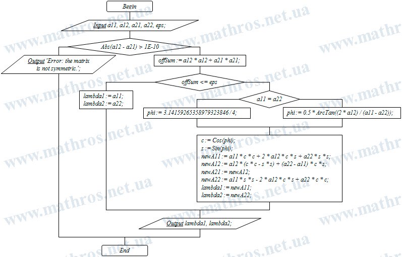
If you are interested in programming, the rotation method can be viewed not only as a set of formulas but also as a ready-made basis for a small computational algorithm. The flowchart below shows the logic of a program for finding the eigenvalues of a symmetric (2\times 2) matrix: from entering the matrix elements to checking symmetry, calculating the rotation angle, and displaying the final result.
Try to implement this algorithm in your favorite programming language — Pascal, Python, C++, JavaScript, or any other language. This will help you better see how the theoretical method turns into a practical tool for numerical calculations.