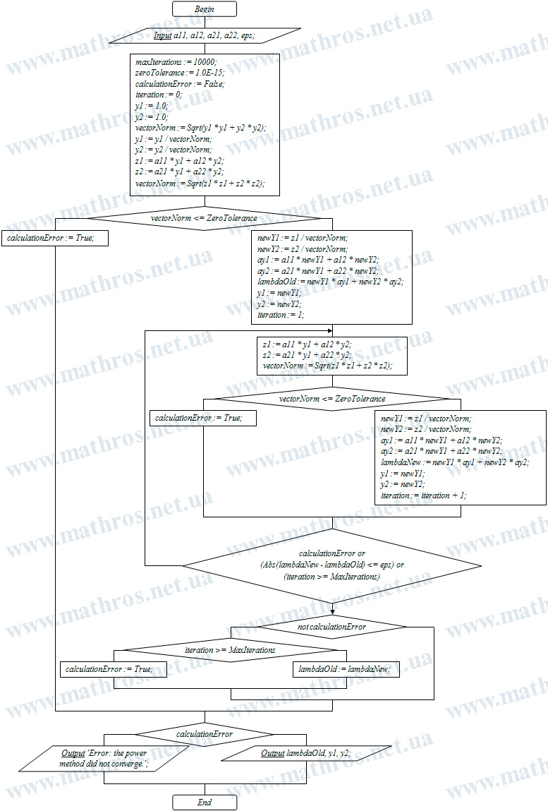
The power method is one of the simplest iterative methods for approximating the dominant eigenvalue of a matrix and its corresponding eigenvector.
The main idea of the method is to repeatedly multiply an initial vector by the given matrix. During this process, the resulting vectors gradually approach the line spanned by the eigenvector associated with the dominant eigenvalue. Let us examine the conditions under which this happens and see how the corresponding iterative process works.
Dominant Eigenvalue of a Matrix: What the Method Actually Finds
Let \( A \) be a square matrix of order \( n \):
\[
A=
\begin{pmatrix}
a_{11} & a_{12} & \dots & a_{1n}\\
a_{21} & a_{22} & \dots & a_{2n}\\
\vdots & \vdots & \ddots & \vdots\\
a_{n1} & a_{n2} & \dots & a_{nn}
\end{pmatrix}.
\]
Suppose that the matrix \( A \) has a complete set of linearly independent eigenvectors and that its eigenvalues are ordered by their absolute values as follows:
\[
|\lambda_1|>|\lambda_2|\geq|\lambda_3|\geq\dots\geq|\lambda_n|.
\]
The eigenvalue \( \lambda_1 \) is called the dominant eigenvalue. Its absolute value is greater than the absolute values of all the other eigenvalues of the matrix:
\[
|\lambda_1|=\max_{1\leq i\leq n}|\lambda_i|.
\]
For the standard power method to converge, the dominant eigenvalue must be unique in absolute value:
\[
|\lambda_1|>|\lambda_2|.
\]
At the same time, the eigenvalues \( \lambda_2,\lambda_3,\dots,\lambda_n \) may have equal absolute values. The important condition is that none of them has the same absolute value as \( \lambda_1 \).
When several eigenvalues have the same largest absolute value, the standard power method may fail to converge to one specific eigenvector. In this case, the behavior of the iterative vectors depends on the initial approximation and the relationship between the corresponding eigenvalues.
Let \( x_1,x_2,\dots,x_n \) be the eigenvectors of the matrix \( A \) corresponding to the eigenvalues \( \lambda_1,\lambda_2,\dots,\lambda_n \). By the definition of an eigenvalue, we have
\[
A\cdot x_i=\lambda_i\cdot x_i,\qquad i=1,2,\dots,n.
\]
Multiply both sides of this equality by the matrix \( A \) again:
\[
A^2\cdot x_i=A\cdot\left(\lambda_i\cdot x_i\right)=\lambda_i\cdot A\cdot x_i=\lambda_i^2\cdot x_i.
\]
Continuing this process, after \( k \) multiplications, we obtain
\[
A^k\cdot x_i=\lambda_i^k\cdot x_i.
\]
Therefore, raising a matrix to a power raises its eigenvalues to the same power. This property is the foundation of the power method.
Power Method: How the Iterative Process Works
First, choose a nonzero initial vector \( y^{(0)} \). For example, we can take
\[
y^{(0)}
=
\begin{pmatrix}
1\\
1\\
\vdots\\
1
\end{pmatrix}.
\]
Since the eigenvectors of the matrix \( A \) form a basis, the initial vector can be expressed as their linear combination:
\[
y^{(0)}=c_1\cdot x_1+c_2\cdot x_2+\dots+c_n\cdot x_n.
\]
For the method to converge to the eigenvector \( x_1 \), which corresponds to the dominant eigenvalue \( \lambda_1 \), the coefficient of \( x_1 \) must not be zero: \( c_1\neq 0 \). If \( c_1=0 \), the eigenvector \( x_1 \) is not included in the expansion of the initial vector. In that case, repeated multiplication by the matrix \( A \) will not produce an iterative vector aligned with the eigenvector \( x_1 \).
After choosing the initial vector, we repeatedly multiply it by the matrix \( A \):
\[
\begin{gathered}
y^{(1)}=A\cdot y^{(0)},\\[4pt]
y^{(2)}=A\cdot y^{(1)},\\[4pt]
\dots\\[4pt]
y^{(k)}=A\cdot y^{(k-1)}.
\end{gathered}
\]
For the second iteration, we have
\[
y^{(2)}=A\cdot y^{(1)}=A\cdot A\cdot y^{(0)}=A^2\cdot y^{(0)}.
\]
Similarly, at the \( k \)-th iteration,
\[
y^{(k)}=A\cdot y^{(k-1)}=A^k\cdot y^{(0)}.
\]
The algorithm is called the power method because it uses successive powers of the matrix.
An approximate value of \( \lambda_1 \) can be calculated using the ratio of the corresponding components of two consecutive vectors:
\[
\lambda_1^{(k)}=\frac{y_j^{(k)}}{y_j^{(k-1)}}.
\]
Here, \( y_j^{(k-1)} \) and \( y_j^{(k)} \) are the components with the same index \( j \) in the vectors \( y^{(k-1)} \) and \( y^{(k)} \).
The complete iterative process can be written as follows:
\[
\begin{gathered}
y^{(1)}=A\cdot y^{(0)},
\qquad
\lambda_1^{(1)}=\frac{y_j^{(1)}}{y_j^{(0)}},\\[4pt]
y^{(2)}=A\cdot y^{(1)},
\qquad
\lambda_1^{(2)}=\frac{y_j^{(2)}}{y_j^{(1)}},\\[4pt]
\dots,
\qquad
\dots,\\[4pt]
y^{(k)}=A\cdot y^{(k-1)},
\qquad
\lambda_1^{(k)}=\frac{y_j^{(k)}}{y_j^{(k-1)}}.
\end{gathered}
\]
The index \( j \) should be chosen so that the denominator \( y_j^{(k-1)} \) is not zero and is not too small in absolute value. Otherwise, the division may be impossible or inaccurate.
In practice, the component with the largest absolute value is often used:
\[
|y_j^{(k-1)}|=\max_{1\leq i\leq n}|y_i^{(k-1)}|.
\]
This choice reduces the risk of dividing by a small number.
Convergence of the Power Method: Why the Iterations Approach the Desired Eigenvector
Substitute the expansion of the initial vector into the general iteration formula:
\[
y^{(k)}=A^k\cdot y^{(0)}.
\]
Since
\[
y^{(0)}=c_1\cdot x_1+c_2\cdot x_2+\dots+c_n\cdot x_n,
\]
we obtain
\[
y^{(k)}=A^k\cdot\left(c_1\cdot x_1+c_2\cdot x_2+\dots+c_n\cdot x_n\right)=c_1\cdot A^k\cdot x_1+c_2\cdot A^k\cdot x_2+\dots+c_n\cdot A^k\cdot x_n.
\]
Now use the property
\[
A^k\cdot x_i=\lambda_i^k\cdot x_i.
\]
Then
\[
y^{(k)}=c_1\cdot\lambda_1^k\cdot x_1+c_2\cdot\lambda_2^k\cdot x_2+\dots+c_n\cdot\lambda_n^k\cdot x_n.
\]
Factor out \( \lambda_1^k \):
\[
y^{(k)}
=
\lambda_1^k\cdot
\left(
c_1\cdot x_1+
c_2\cdot
\left(
\frac{\lambda_2}{\lambda_1}
\right)^k
\cdot x_2+
\dots+
c_n\cdot
\left(
\frac{\lambda_n}{\lambda_1}
\right)^k
\cdot x_n
\right).
\]
Since \( \lambda_1 \) is the unique dominant eigenvalue, the following inequality holds for every \( i=2,3,\dots,n \):
\[
\left|\frac{\lambda_i}{\lambda_1}\right|<1.
\]
Therefore, as \( k \) increases,
\[
\left(\frac{\lambda_i}{\lambda_1}\right)^k\to 0,\qquad i=2,3,\dots,n.
\]
This means that the influence of the terms associated with the eigenvectors \( x_2,x_3,\dots,x_n \) gradually decreases. For a sufficiently large value of \( k \), the main contribution to the vector \( y^{(k)} \) comes from the term associated with \( x_1 \):
\[
y^{(k)}\approx c_1\cdot\lambda_1^k\cdot x_1.
\]
It follows that the direction of the iterative vector gradually approaches the direction of the eigenvector \( x_1 \). At the same time, the ratio of the corresponding components of two consecutive vectors approaches the dominant eigenvalue:
\[
\frac{y_j^{(k)}}{y_j^{(k-1)}}\to\lambda_1.
\]
It is important to distinguish between the iterative vector approaching the line spanned by \( x_1 \) and its components converging to finite values.
If \( |\lambda_1|>1 \), the absolute values of the components of \( y^{(k)} \) may grow without limit. If \( |\lambda_1|<1 \), they may approach zero. However, the ratios between the components become stable, so the vector aligns more and more accurately with the line spanned by \( x_1 \).
The convergence rate is determined by the ratio
\[
\frac{|\lambda_2|}{|\lambda_1|}.
\]
The smaller this ratio is, the faster the influence of the terms associated with the other eigenvalues decreases. If \( |\lambda_2| \) is close to \( |\lambda_1| \), convergence will be slow.
The iterative process can be stopped when two consecutive approximations of the eigenvalue differ by no more than the required accuracy:
\[
\left|\lambda_1^{(k)}-\lambda_1^{(k-1)}\right|\leq\varepsilon.
\]
Here, \( \varepsilon \) is the required calculation accuracy.
For a more reliable check, we can also use the residual:
\[
r^{(k)}=A\cdot y^{(k)}-\lambda_1^{(k)}\cdot y^{(k)}.
\]
If the vector \( y^{(k)} \) is not normalized, it is better to use the relative criterion:
\[
\frac{\left\|A\cdot y^{(k)}-\lambda_1^{(k)}\cdot y^{(k)}\right\|}{\left\|y^{(k)}\right\|}\leq\varepsilon.
\]
This criterion shows how accurately the calculated approximations satisfy the eigenvalue equation
\[
A\cdot y=\lambda\cdot y.
\]
Normalizing the Iterative Vector: How to Avoid Numerical Problems
In the standard power method, the components of the vector may become too large or too small. This can cause problems during computer calculations.
To keep the algorithm numerically stable, the resulting vector is normalized after each multiplication. First, calculate an auxiliary vector:
\[
z^{(k)}=A\cdot y^{(k-1)}.
\]
Next, find an approximation of the eigenvalue:
\[
\lambda_1^{(k)}=\frac{z_j^{(k)}}{y_j^{(k-1)}}.
\]
After that, normalize the vector \( z^{(k)} \) so that it has unit norm:
\[
y^{(k)}=\frac{z^{(k)}}{\left\|z^{(k)}\right\|}.
\]
Therefore, the power method with normalization can be written as
\[
z^{(k)}=A\cdot y^{(k-1)},\qquad \lambda_1^{(k)}=\frac{z_j^{(k)}}{y_j^{(k-1)}},\qquad y^{(k)}=\frac{z^{(k)}}{\left\|z^{(k)}\right\|}.
\]
It is also useful to normalize the initial vector. If a nonzero vector \( \widetilde{y}^{(0)} \) is chosen initially, then
\[
y^{(0)}=\frac{\widetilde{y}^{(0)}}{\left\|\widetilde{y}^{(0)}\right\|}.
\]
In this case,
\[
\left\|y^{(0)}\right\|=1.
\]
Normalization changes the length of a vector but keeps it on the same line passing through the origin. Therefore, it does not affect the basic principle of the power method.
If the dominant eigenvalue is negative, the normalized vectors may alternate in sign:
\[
x_1,\quad -x_1,\quad x_1,\quad -x_1,\quad\dots
\]
This is not an error because the vectors \( x_1 \) and \( -x_1 \) lie on the same line and correspond to the same eigenvalue.
In practice, another version of the method is also used in which the approximate eigenvalue is calculated using the inner product. First, perform the multiplication and normalization:
\[
z^{(k)}=A\cdot y^{(k-1)},\qquad y^{(k)}=\frac{z^{(k)}}{\left\|z^{(k)}\right\|}.
\]
Then calculate the approximate eigenvalue:
\[
\lambda_1^{(k)}=\frac{\left(y^{(k)},A\cdot y^{(k)}\right)}{\left(y^{(k)},y^{(k)}\right)}.
\]
This expression is called the Rayleigh quotient.
Since the vector \( y^{(k)} \) is normalized, we have \( \left(y^{(k)},y^{(k)}\right)=1 \). Therefore, the formula becomes
\[
\lambda_1^{(k)}=\left(y^{(k)},A\cdot y^{(k)}\right).
\]
Thus, the power method gradually isolates the part of the initial vector associated with the dominant eigenvalue. Normalization makes it possible to carry out this process without the components of the iterative vector becoming excessively large or small. As a result, we obtain an approximation of the eigenvalue with the largest absolute value and its corresponding eigenvector.
Dominant Eigenvalue of a Matrix: Power Method in Practice
Now let us see how the power method works for matrices of different orders. In each example, we will normalize the iterative vector, calculate an approximate eigenvalue using the Rayleigh quotient, and compare two consecutive approximations.
Example 1. Find the dominant eigenvalue of the matrix
\[
A=
\begin{pmatrix}
4 & 1\\
1 & 2
\end{pmatrix}
\]
and the corresponding eigenvector to an accuracy of \( \varepsilon=0.1 \)
Choose the following vector as the initial approximation:
\[
\widetilde{y}^{(0)}
=
\begin{pmatrix}
1\\
1
\end{pmatrix}.
\]
Calculate its Euclidean norm:
\[
\left\|\widetilde{y}^{(0)}\right\|=\sqrt{1^2+1^2}=\sqrt{2}.
\]
Normalize the initial vector:
\[
y^{(0)}
=
\frac{\widetilde{y}^{(0)}}{\left\|\widetilde{y}^{(0)}\right\|}
=
\frac{1}{\sqrt{2}}
\cdot
\begin{pmatrix}
1\\
1
\end{pmatrix}
\approx
\begin{pmatrix}
0.7071\\
0.7071
\end{pmatrix}.
\]
Perform the first iteration:
\[
z^{(1)}=A\cdot y^{(0)}.
\]
Substitute the matrix and the initial vector:
\[
z^{(1)}
=
\begin{pmatrix}
4 & 1\\
1 & 2
\end{pmatrix}
\cdot
\begin{pmatrix}
0.7071\\
0.7071
\end{pmatrix}.
\]
Calculate the components of the vector:
\[
z^{(1)}
=
\begin{pmatrix}
4\cdot 0.7071+1\cdot 0.7071\\
1\cdot 0.7071+2\cdot 0.7071
\end{pmatrix}
\approx
\begin{pmatrix}
3.5355\\
2.1213
\end{pmatrix}.
\]
Find the norm of the resulting vector:
\[
\left\|z^{(1)}\right\|=\sqrt{3.5355^2+2.1213^2}\approx 4.1231.
\]
Normalize the vector:
\[
y^{(1)}
=
\frac{z^{(1)}}{\left\|z^{(1)}\right\|}
=
\frac{1}{4.1231}
\cdot
\begin{pmatrix}
3.5355\\
2.1213
\end{pmatrix}
\approx
\begin{pmatrix}
0.8575\\
0.5145
\end{pmatrix}.
\]
Now calculate the product \( A\cdot y^{(1)} \):
\[
A\cdot y^{(1)}
=
\begin{pmatrix}
4 & 1\\
1 & 2
\end{pmatrix}
\cdot
\begin{pmatrix}
0.8575\\
0.5145
\end{pmatrix}.
\]
We obtain
\[
A\cdot y^{(1)}
=
\begin{pmatrix}
4\cdot 0.8575+1\cdot 0.5145\\
1\cdot 0.8575+2\cdot 0.5145
\end{pmatrix}
\approx
\begin{pmatrix}
3.9445\\
1.8865
\end{pmatrix}.
\]
Find the first approximation of the eigenvalue using the Rayleigh quotient:
\[
\lambda_1^{(1)}=\left(y^{(1)},A\cdot y^{(1)}\right).
\]
Since the vector \( y^{(1)} \) has unit norm, we obtain
\[
\lambda_1^{(1)}=0.8575\cdot 3.9445+0.5145\cdot 1.8865\approx 4.3529.
\]
Move on to the second iteration. The product \( A\cdot y^{(1)} \), which has already been calculated, is the vector \( z^{(2)} \):
\[
z^{(2)}
=
\begin{pmatrix}
3.9445\\
1.8865
\end{pmatrix}.
\]
Its norm is
\[
\left\|z^{(2)}\right\|=\sqrt{3.9445^2+1.8865^2}\approx 4.3724.
\]
Therefore,
\[
y^{(2)}
=
\frac{z^{(2)}}{\left\|z^{(2)}\right\|}
=
\frac{1}{4.3724}
\cdot
\begin{pmatrix}
3.9445\\
1.8865
\end{pmatrix}
\approx
\begin{pmatrix}
0.9021\\
0.4315
\end{pmatrix}.
\]
Calculate the next product:
\[
A\cdot y^{(2)}
=
\begin{pmatrix}
4 & 1\\
1 & 2
\end{pmatrix}
\cdot
\begin{pmatrix}
0.9021\\
0.4315
\end{pmatrix}.
\]
We obtain
\[
A\cdot y^{(2)}
=
\begin{pmatrix}
4\cdot 0.9021+1\cdot 0.4315\\
1\cdot 0.9021+2\cdot 0.4315
\end{pmatrix}
\approx
\begin{pmatrix}
4.04\\
1.765
\end{pmatrix}.
\]
The second approximation of the eigenvalue is
\[
\lambda_1^{(2)}=\left(y^{(2)},A\cdot y^{(2)}\right)=0.9021\cdot 4.04+0.4315\cdot 1.765\approx 4.4062.
\]
Check the stopping condition:
\[
\left|\lambda_1^{(2)}-\lambda_1^{(1)}\right|=|4.4062-4.3529|=0.0533.
\]
Since
\[
0.0533\leq 0.1,
\]
we stop the iterative process.
Therefore, the dominant eigenvalue of the matrix is approximately
\[
\lambda_1\approx 4.4062.
\]
We take the last normalized iterative vector as the approximate eigenvector corresponding to the estimated eigenvalue:
\[
x_1
\approx
\begin{pmatrix}
0.9021\\
0.4315
\end{pmatrix}.
\]
Example 2. Find the dominant eigenvalue of the matrix
\[
A=
\begin{pmatrix}
5 & 1 & 0\\
1 & 3 & 1\\
0 & 1 & 2
\end{pmatrix}
\]
and the corresponding eigenvector to an accuracy of \( \varepsilon=0.1 \)
Choose the initial vector
\[
\widetilde{y}^{(0)}
=
\begin{pmatrix}
1\\
1\\
1
\end{pmatrix}.
\]
Its Euclidean norm is
\[
\left\|\widetilde{y}^{(0)}\right\|=\sqrt{1^2+1^2+1^2}=\sqrt{3}.
\]
Normalize the initial vector:
\[
y^{(0)}
=
\frac{\widetilde{y}^{(0)}}{\left\|\widetilde{y}^{(0)}\right\|}
=
\frac{1}{\sqrt{3}}
\cdot
\begin{pmatrix}
1\\
1\\
1
\end{pmatrix}
\approx
\begin{pmatrix}
0.5774\\
0.5774\\
0.5774
\end{pmatrix}.
\]
Perform the first iteration:
\[
z^{(1)}=A\cdot y^{(0)}.
\]
Substitute the matrix and the vector:
\[
z^{(1)}
=
\begin{pmatrix}
5 & 1 & 0\\
1 & 3 & 1\\
0 & 1 & 2
\end{pmatrix}
\cdot
\begin{pmatrix}
0.5774\\
0.5774\\
0.5774
\end{pmatrix}.
\]
Calculate the components:
\[
z^{(1)}
=
\begin{pmatrix}
5\cdot 0.5774+1\cdot 0.5774+0\cdot 0.5774\\
1\cdot 0.5774+3\cdot 0.5774+1\cdot 0.5774\\
0\cdot 0.5774+1\cdot 0.5774+2\cdot 0.5774
\end{pmatrix}
\approx
\begin{pmatrix}
3.4641\\
2.8868\\
1.7321
\end{pmatrix}.
\]
Find the norm:
\[
\left\|z^{(1)}\right\|=\sqrt{3.4641^2+2.8868^2+1.7321^2}\approx 4.8305.
\]
Then
\[
y^{(1)}
=
\frac{z^{(1)}}{\left\|z^{(1)}\right\|}
=
\frac{1}{4.8305}
\cdot
\begin{pmatrix}
3.4641\\
2.8868\\
1.7321
\end{pmatrix}
\approx
\begin{pmatrix}
0.7171\\
0.5976\\
0.3586
\end{pmatrix}.
\]
Find the product \( A\cdot y^{(1)} \):
\[
A\cdot y^{(1)}
=
\begin{pmatrix}
5 & 1 & 0\\
1 & 3 & 1\\
0 & 1 & 2
\end{pmatrix}
\cdot
\begin{pmatrix}
0.7171\\
0.5976\\
0.3586
\end{pmatrix}.
\]
After multiplication, we have
\[
A\cdot y^{(1)}
=
\begin{pmatrix}
5\cdot 0.7171+1\cdot 0.5976+0\cdot 0.3586\\
1\cdot 0.7171+3\cdot 0.5976+1\cdot 0.3586\\
0\cdot 0.7171+1\cdot 0.5976+2\cdot 0.3586
\end{pmatrix}
\approx
\begin{pmatrix}
4.1833\\
2.8685\\
1.3148
\end{pmatrix}.
\]
Calculate the first approximation of the eigenvalue:
\[
\lambda_1^{(1)}=\left(y^{(1)},A\cdot y^{(1)}\right)=0.7171\cdot 4.1833+0.5976\cdot 2.8685+0.3586\cdot 1.3148\approx 5.1857.
\]
Move on to the second iteration:
\[
z^{(2)}
=
\begin{pmatrix}
4.1833\\
2.8685\\
1.3148
\end{pmatrix}.
\]
Find the norm:
\[
\left\|z^{(2)}\right\|=\sqrt{4.1833^2+2.8685^2+1.3148^2}\approx 5.24.
\]
Normalize the vector:
\[
y^{(2)}
=
\frac{z^{(2)}}{\left\|z^{(2)}\right\|}
=
\frac{1}{5.24}
\cdot
\begin{pmatrix}
4.1833\\
2.8685\\
1.3148
\end{pmatrix}
\approx
\begin{pmatrix}
0.7983\\
0.5474\\
0.2509
\end{pmatrix}.
\]
Calculate
\[
A\cdot y^{(2)}
=
\begin{pmatrix}
5 & 1 & 0\\
1 & 3 & 1\\
0 & 1 & 2
\end{pmatrix}
\cdot
\begin{pmatrix}
0.7983\\
0.5474\\
0.2509
\end{pmatrix}.
\]
We obtain
\[
A\cdot y^{(2)}
=
\begin{pmatrix}
5\cdot 0.7983+1\cdot 0.5474+0\cdot 0.2509\\
1\cdot 0.7983+3\cdot 0.5474+1\cdot 0.2509\\
0\cdot 0.7983+1\cdot 0.5474+2\cdot 0.2509
\end{pmatrix}
\approx
\begin{pmatrix}
4.5392\\
2.6916\\
1.0493
\end{pmatrix}.
\]
The second approximation of the eigenvalue is
\[
\lambda_1^{(2)}=\left(y^{(2)},A\cdot y^{(2)}\right)=0.7983\cdot 4.5392+0.5474\cdot 2.6916+0.2509\cdot 1.0493\approx 5.3606.
\]
Check the stopping condition:
\[
\left|\lambda_1^{(2)}-\lambda_1^{(1)}\right|=|5.3606-5.1857|=0.1749.
\]
Since
\[
0.1749>0.1,
\]
we need to perform one more iteration.
We have
\[
z^{(3)}
=
\begin{pmatrix}
4.5392\\
2.6916\\
1.0493
\end{pmatrix}.
\]
Find the norm:
\[
\left\|z^{(3)}\right\|=\sqrt{4.5392^2+2.6916^2+1.0493^2}\approx 5.3805.
\]
Then
\[
y^{(3)}
=
\frac{z^{(3)}}{\left\|z^{(3)}\right\|}
=
\frac{1}{5.3805}
\cdot
\begin{pmatrix}
4.5392\\
2.6916\\
1.0493
\end{pmatrix}
\approx
\begin{pmatrix}
0.8436\\
0.5002\\
0.195
\end{pmatrix}.
\]
Calculate
\[
A\cdot y^{(3)}
=
\begin{pmatrix}
5 & 1 & 0\\
1 & 3 & 1\\
0 & 1 & 2
\end{pmatrix}
\cdot
\begin{pmatrix}
0.8436\\
0.5002\\
0.195
\end{pmatrix}.
\]
We obtain
\[
A\cdot y^{(3)}
=
\begin{pmatrix}
5\cdot 0.8436+1\cdot 0.5002+0\cdot 0.195\\
1\cdot 0.8436+3\cdot 0.5002+1\cdot 0.195\\
0\cdot 0.8436+1\cdot 0.5002+2\cdot 0.195
\end{pmatrix}
\approx
\begin{pmatrix}
4.7184\\
2.5394\\
0.8903
\end{pmatrix}.
\]
The third approximation of the eigenvalue is
\[
\lambda_1^{(3)}=\left(y^{(3)},A\cdot y^{(3)}\right)=0.8436\cdot 4.7184+0.5002\cdot 2.5394+0.195\cdot 0.8903\approx 5.4246.
\]
Check the stopping condition:
\[
\left|\lambda_1^{(3)}-\lambda_1^{(2)}\right|=|5.4246-5.3606|=0.064.
\]
Since
\[
0.064\leq 0.1,
\]
we stop the iterative process.
Therefore, the dominant eigenvalue of the matrix is approximately
\[
\lambda_1\approx 5.4246.
\]
We take the last normalized iterative vector as the approximate eigenvector corresponding to the estimated eigenvalue:
\[
x_1
\approx
\begin{pmatrix}
0.8436\\
0.5002\\
0.195
\end{pmatrix}.
\]
Example 3. Find the dominant eigenvalue of the matrix
\[
A=
\begin{pmatrix}
6 & 1 & 0 & 0\\
1 & 4 & 1 & 0\\
0 & 1 & 3 & 1\\
0 & 0 & 1 & 2
\end{pmatrix}
\]
and the corresponding eigenvector to an accuracy of \( \varepsilon=0.1 \)
Choose the initial vector
\[
\widetilde{y}^{(0)}
=
\begin{pmatrix}
1\\
1\\
1\\
1
\end{pmatrix}.
\]
Its Euclidean norm is
\[
\left\|\widetilde{y}^{(0)}\right\|=\sqrt{1^2+1^2+1^2+1^2}=2.
\]
Therefore, the normalized initial vector is
\[
y^{(0)}
=
\frac{\widetilde{y}^{(0)}}{\left\|\widetilde{y}^{(0)}\right\|}
=
\frac{1}{2}
\cdot
\begin{pmatrix}
1\\
1\\
1\\
1
\end{pmatrix}
=
\begin{pmatrix}
0.5\\
0.5\\
0.5\\
0.5
\end{pmatrix}.
\]
Perform the first iteration:
\[
z^{(1)}=A\cdot y^{(0)}.
\]
Substitute the matrix and the vector:
\[
z^{(1)}
=
\begin{pmatrix}
6 & 1 & 0 & 0\\
1 & 4 & 1 & 0\\
0 & 1 & 3 & 1\\
0 & 0 & 1 & 2
\end{pmatrix}
\cdot
\begin{pmatrix}
0.5\\
0.5\\
0.5\\
0.5
\end{pmatrix}.
\]
After multiplication, we obtain
\[
z^{(1)}
=
\begin{pmatrix}
6\cdot 0.5+1\cdot 0.5+0\cdot 0.5+0\cdot 0.5\\
1\cdot 0.5+4\cdot 0.5+1\cdot 0.5+0\cdot 0.5\\
0\cdot 0.5+1\cdot 0.5+3\cdot 0.5+1\cdot 0.5\\
0\cdot 0.5+0\cdot 0.5+1\cdot 0.5+2\cdot 0.5
\end{pmatrix}
=
\begin{pmatrix}
3.5\\
3\\
2.5\\
1.5
\end{pmatrix}.
\]
Find the norm:
\[
\left\|z^{(1)}\right\|=\sqrt{3.5^2+3^2+2.5^2+1.5^2}\approx 5.4544.
\]
Then
\[
y^{(1)}
=
\frac{z^{(1)}}{\left\|z^{(1)}\right\|}
=
\frac{1}{5.4544}
\cdot
\begin{pmatrix}
3.5\\
3\\
2.5\\
1.5
\end{pmatrix}
\approx
\begin{pmatrix}
0.6417\\
0.55\\
0.4583\\
0.275
\end{pmatrix}.
\]
Calculate the product
\[
A\cdot y^{(1)}
=
\begin{pmatrix}
6 & 1 & 0 & 0\\
1 & 4 & 1 & 0\\
0 & 1 & 3 & 1\\
0 & 0 & 1 & 2
\end{pmatrix}
\cdot
\begin{pmatrix}
0.6417\\
0.55\\
0.4583\\
0.275
\end{pmatrix}.
\]
We have
\[
A\cdot y^{(1)}
=
\begin{pmatrix}
6\cdot 0.6417+1\cdot 0.55+0\cdot 0.4583+0\cdot 0.275\\
1\cdot 0.6417+4\cdot 0.55+1\cdot 0.4583+0\cdot 0.275\\
0\cdot 0.6417+1\cdot 0.55+3\cdot 0.4583+1\cdot 0.275\\
0\cdot 0.6417+0\cdot 0.55+1\cdot 0.4583+2\cdot 0.275
\end{pmatrix}
\approx
\begin{pmatrix}
4.4002\\
3.3001\\
2.2001\\
1.0084
\end{pmatrix}.
\]
The first approximation of the eigenvalue is
\[
\lambda_1^{(1)}=\left(y^{(1)},A\cdot y^{(1)}\right)=0.6417\cdot 4.4002+0.55\cdot 3.3001+0.4583\cdot 2.2001+0.275\cdot 1.0084\approx 5.9244.
\]
At the second iteration, we have
\[
z^{(2)}
=
\begin{pmatrix}
4.4002\\
3.3001\\
2.2001\\
1.0084
\end{pmatrix}.
\]
Its norm is
\[
\left\|z^{(2)}\right\|=\sqrt{4.4002^2+3.3001^2+2.2001^2+1.0084^2}\approx 6.0091.
\]
Therefore,
\[
y^{(2)}
=
\frac{z^{(2)}}{\left\|z^{(2)}\right\|}
=
\frac{1}{6.0091}
\cdot
\begin{pmatrix}
4.4002\\
3.3001\\
2.2001\\
1.0084
\end{pmatrix}
\approx
\begin{pmatrix}
0.7322\\
0.5492\\
0.3661\\
0.1678
\end{pmatrix}.
\]
Calculate
\[
A\cdot y^{(2)}
=
\begin{pmatrix}
6 & 1 & 0 & 0\\
1 & 4 & 1 & 0\\
0 & 1 & 3 & 1\\
0 & 0 & 1 & 2
\end{pmatrix}
\cdot
\begin{pmatrix}
0.7322\\
0.5492\\
0.3661\\
0.1678
\end{pmatrix}.
\]
After multiplication, we obtain
\[
A\cdot y^{(2)}
=
\begin{pmatrix}
6\cdot 0.7322+1\cdot 0.5492+0\cdot 0.3661+0\cdot 0.1678\\
1\cdot 0.7322+4\cdot 0.5492+1\cdot 0.3661+0\cdot 0.1678\\
0\cdot 0.7322+1\cdot 0.5492+3\cdot 0.3661+1\cdot 0.1678\\
0\cdot 0.7322+0\cdot 0.5492+1\cdot 0.3661+2\cdot 0.1678
\end{pmatrix}
\approx
\begin{pmatrix}
4.9427\\
3.2951\\
1.8154\\
0.7017
\end{pmatrix}.
\]
The second approximation of the eigenvalue is
\[
\lambda_1^{(2)}=\left(y^{(2)},A\cdot y^{(2)}\right)=0.7322\cdot 4.9427+0.5492\cdot 3.2951+0.3661\cdot 1.8154+0.1678\cdot 0.7017\approx 6.2113.
\]
Check the stopping condition:
\[
\left|\lambda_1^{(2)}-\lambda_1^{(1)}\right|=|6.2113-5.9244|=0.2869.
\]
Since
\[
0.2869>0.1,
\]
we continue the calculations.
At the third iteration,
\[
z^{(3)}
=
\begin{pmatrix}
4.9427\\
3.2951\\
1.8154\\
0.7017
\end{pmatrix}.
\]
Find the norm:
\[
\left\|z^{(3)}\right\|=\sqrt{4.9427^2+3.2951^2+1.8154^2+0.7017^2}\approx 6.2511.
\]
Then
\[
y^{(3)}
=
\frac{z^{(3)}}{\left\|z^{(3)}\right\|}
=
\frac{1}{6.2511}
\cdot
\begin{pmatrix}
4.9427\\
3.2951\\
1.8154\\
0.7017
\end{pmatrix}
\approx
\begin{pmatrix}
0.7907\\
0.5271\\
0.2904\\
0.1123
\end{pmatrix}.
\]
Calculate the next product:
\[
A\cdot y^{(3)}
=
\begin{pmatrix}
6 & 1 & 0 & 0\\
1 & 4 & 1 & 0\\
0 & 1 & 3 & 1\\
0 & 0 & 1 & 2
\end{pmatrix}
\cdot
\begin{pmatrix}
0.7907\\
0.5271\\
0.2904\\
0.1123
\end{pmatrix}.
\]
We obtain
\[
A\cdot y^{(3)}
=
\begin{pmatrix}
6\cdot 0.7907+1\cdot 0.5271+0\cdot 0.2904+0\cdot 0.1123\\
1\cdot 0.7907+4\cdot 0.5271+1\cdot 0.2904+0\cdot 0.1123\\
0\cdot 0.7907+1\cdot 0.5271+3\cdot 0.2904+1\cdot 0.1123\\
0\cdot 0.7907+0\cdot 0.5271+1\cdot 0.2904+2\cdot 0.1123
\end{pmatrix}
\approx
\begin{pmatrix}
5.2713\\
3.1896\\
1.5106\\
0.5149
\end{pmatrix}.
\]
The third approximation of the eigenvalue is
\[
\lambda_1^{(3)}=\left(y^{(3)},A\cdot y^{(3)}\right)=0.7907\cdot 5.2713+0.5271\cdot 3.1896+0.2904\cdot 1.5106+0.1123\cdot 0.5149\approx 6.3458.
\]
Check the difference:
\[
\left|\lambda_1^{(3)}-\lambda_1^{(2)}\right|=|6.3458-6.2113|=0.1345.
\]
Since
\[
0.1345>0.1,
\]
we need to perform the fourth iteration.
We have
\[
z^{(4)}
=
\begin{pmatrix}
5.2713\\
3.1896\\
1.5106\\
0.5149
\end{pmatrix}.
\]
Its norm is
\[
\left\|z^{(4)}\right\|=\sqrt{5.2713^2+3.1896^2+1.5106^2+0.5149^2}\approx 6.3645.
\]
Therefore,
\[
y^{(4)}
=
\frac{z^{(4)}}{\left\|z^{(4)}\right\|}
=
\frac{1}{6.3645}
\cdot
\begin{pmatrix}
5.2713\\
3.1896\\
1.5106\\
0.5149
\end{pmatrix}
\approx
\begin{pmatrix}
0.8282\\
0.5012\\
0.2373\\
0.0809
\end{pmatrix}.
\]
Calculate
\[
A\cdot y^{(4)}
=
\begin{pmatrix}
6 & 1 & 0 & 0\\
1 & 4 & 1 & 0\\
0 & 1 & 3 & 1\\
0 & 0 & 1 & 2
\end{pmatrix}
\cdot
\begin{pmatrix}
0.8282\\
0.5012\\
0.2373\\
0.0809
\end{pmatrix}.
\]
After multiplication, we have
\[
A\cdot y^{(4)}
=
\begin{pmatrix}
6\cdot 0.8282+1\cdot 0.5012+0\cdot 0.2373+0\cdot 0.0809\\
1\cdot 0.8282+4\cdot 0.5012+1\cdot 0.2373+0\cdot 0.0809\\
0\cdot 0.8282+1\cdot 0.5012+3\cdot 0.2373+1\cdot 0.0809\\
0\cdot 0.8282+0\cdot 0.5012+1\cdot 0.2373+2\cdot 0.0809
\end{pmatrix}
\approx
\begin{pmatrix}
5.4705\\
3.0702\\
1.2941\\
0.3992
\end{pmatrix}.
\]
The fourth approximation of the eigenvalue is
\[
\lambda_1^{(4)}=\left(y^{(4)},A\cdot y^{(4)}\right)=0.8282\cdot 5.4705+0.5012\cdot 3.0702+0.2373\cdot 1.2941+0.0809\cdot 0.3992\approx 6.4089.
\]
Check the stopping condition:
\[
\left|\lambda_1^{(4)}-\lambda_1^{(3)}\right|=|6.4089-6.3458|=0.0631.
\]
Since
\[
0.0631\leq 0.1,
\]
we stop the iterative process.
Therefore, the dominant eigenvalue of the matrix is approximately
\[
\lambda_1\approx 6.4089.
\]
We take the last normalized iterative vector as the approximate eigenvector corresponding to the estimated eigenvalue:
\[
x_1
\approx
\begin{pmatrix}
0.8282\\
0.5012\\
0.2373\\
0.0809
\end{pmatrix}.
\]
What to Study Next: Methods for Other Eigenvalue Problems
After learning the power method, it is worth moving on to methods that solve other problems in spectral analysis. They will help you find additional eigenvalues and work with matrices that have special structures.
- Deflation Method: How to Find the Second Eigenvalue — This article will show how to calculate the next eigenvalue after finding the dominant eigenvalue.
- Rotation Method: How to Analyze a Symmetric Matrix — The material will explain how successive orthogonal transformations reduce a symmetric matrix to a nearly diagonal form.
- Bisection Method: How to Work with a Tridiagonal Matrix — This article will explain how to narrow the search intervals and approximate the spectrum of a symmetric tridiagonal matrix.
Dominant Eigenvalue of a Matrix: Implement the Algorithm Yourself
If you enjoy programming, try turning the flowchart into a complete program in your favorite programming language. This practice will help you better understand how the power method moves from mathematical formulas to a sequence of calculations. It will also allow you to test the algorithm with different matrices and accuracy values.