Eigenvectors of a matrix can be found in different ways. One such approach is related to the Krylov method. Usually, this method is first used to find the coefficients of the characteristic polynomial. But what should we do next when the eigenvalues have already been found? This is where Krylov vectors can be used once again. They help us construct eigenvectors of a matrix through a special linear combination of already known vectors.
Eigenvectors of a Matrix: What You Need to Know Before Construction
Let a square matrix \( A \) of order \( n \) be given. Also, suppose that the characteristic polynomial of this matrix has already been found. We write it in the form
\[
D(\lambda)
=
\lambda^{n}
+
p_1\cdot\lambda^{n-1}
+
p_2\cdot\lambda^{n-2}
+
\dots
+
p_n.
\]
Next, assume that all roots of this polynomial are distinct. In other words, the matrix has the eigenvalues
\[
\lambda_1,\lambda_2,\lambda_3,\dots,\lambda_n.
\]
Why is this important? Because for distinct eigenvalues, the construction of eigenvectors has a simpler and more convenient form. Each eigenvalue \( \lambda_i \) has a corresponding eigenvector \( x_i \), for which the equality \( A\cdot x_i=\lambda_i\cdot x_i \) holds.
So, our task is the following: for each eigenvalue \( \lambda_i \), we need to construct the corresponding eigenvector. Moreover, we will do this not by directly solving the system \( (A-\lambda_i\cdot E)\cdot x=0 \), but through Krylov vectors.
First, we choose a nonzero initial vector \( y^{(0)} \). Then we construct the following sequence of vectors:
\[
y^{(1)}=A\cdot y^{(0)},
\qquad
y^{(2)}=A\cdot y^{(1)},
\qquad
\dots,
\qquad
y^{(n)}=A\cdot y^{(n-1)}.
\]
In other words, each new vector is obtained by multiplying the previous vector by the matrix \( A \). This gives us the sequence of vectors
\[
y^{(0)},y^{(1)},y^{(2)},\dots,y^{(n)}.
\]
These vectors are called Krylov vectors. Next, they will help us construct the eigenvectors of a matrix.
Krylov Method: How Vectors Are Connected with Eigenvalues
Now let’s look at why Krylov vectors can be used to find eigenvectors. Suppose that the eigenvectors of the matrix \( A \) have the form
\[
x_1,x_2,x_3,\dots,x_n.
\]
Assume that the initial vector \( y^{(0)} \) can be expressed through these eigenvectors:
\[
y^{(0)}
=
c_1\cdot x_1
+
c_2\cdot x_2
+
c_3\cdot x_3
+
\dots
+
c_n\cdot x_n.
\]
Here, \( c_1,c_2,c_3,\dots,c_n \) are some numerical coefficients. Usually, we assume that \( c_i\ne0 \), where \( i=1,2,3,\dots,n \). This means that the initial vector has a nonzero component in the direction of each eigenvector.
Next, we use the main property of an eigenvector. If \( x_i \) is an eigenvector of the matrix \( A \), then \( A\cdot x_i=\lambda_i\cdot x_i \). Therefore, after multiplying \( y^{(0)} \) by the matrix \( A \), we get
\[
y^{(1)}
=
A\cdot y^{(0)}
=
c_1\cdot\lambda_1\cdot x_1
+
c_2\cdot\lambda_2\cdot x_2
+
c_3\cdot\lambda_3\cdot x_3
+
\dots
+
c_n\cdot\lambda_n\cdot x_n.
\]
And what happens with the next vectors? The same principle works here. For example,
\[
y^{(2)}
=
c_1\cdot\lambda_1^2\cdot x_1
+
c_2\cdot\lambda_2^2\cdot x_2
+
c_3\cdot\lambda_3^2\cdot x_3
+
\dots
+
c_n\cdot\lambda_n^2\cdot x_n.
\]
For any number \( k \), we can write the general formula:
\[
y^{(k)}
=
c_1\cdot\lambda_1^k\cdot x_1
+
c_2\cdot\lambda_2^k\cdot x_2
+
c_3\cdot\lambda_3^k\cdot x_3
+
\dots
+
c_n\cdot\lambda_n^k\cdot x_n.
\]
So, each Krylov vector contains the same eigenvectors \( x_1,x_2,\dots,x_n \), but with different powers of the eigenvalues. This is exactly what makes it possible to isolate the required eigenvector. How can we do that? We need to create such a linear combination of Krylov vectors that all extra eigenvectors disappear, and only one remains.
Constructing an Eigenvector: The Role of an Auxiliary Polynomial
For each eigenvalue \( \lambda_i \), we introduce an auxiliary polynomial
\[
Q_i(\lambda)
=
\frac{D(\lambda)}{\lambda-\lambda_i}.
\]
Since \( \lambda_i \) is a root of the characteristic polynomial \( D(\lambda) \), this division of polynomials is possible. The polynomial \( Q_i(\lambda) \) has degree \( n-1 \), so it can be written as follows:
\[
Q_i(\lambda)
=
\lambda^{n-1}
+
q_{1i}\cdot\lambda^{n-2}
+
q_{2i}\cdot\lambda^{n-3}
+
q_{3i}\cdot\lambda^{n-4}
+
\dots
+
q_{n-1,i}.
\]
Now we form a linear combination of Krylov vectors with the same coefficients. Let us denote the constructed vector by \( v_i \):
\[
v_i
=
y^{(n-1)}
+
q_{1i}\cdot y^{(n-2)}
+
q_{2i}\cdot y^{(n-3)}
+
q_{3i}\cdot y^{(n-4)}
+
\dots
+
q_{n-1,i}\cdot y^{(0)}.
\]
Why do we use exactly this combination? Because after substituting the expressions of the vectors \( y^{(0)},y^{(1)},\dots,y^{(n-1)} \) through the eigenvectors, we get
\[
v_i
=
c_1\cdot Q_i(\lambda_1)\cdot x_1
+
c_2\cdot Q_i(\lambda_2)\cdot x_2
+
c_3\cdot Q_i(\lambda_3)\cdot x_3
+
\dots
+
c_n\cdot Q_i(\lambda_n)\cdot x_n.
\]
Now let’s pay attention to the main property of the polynomial \( Q_i(\lambda) \). Since
\[
Q_i(\lambda)
=
\frac{D(\lambda)}{\lambda-\lambda_i},
\]
for all \( j\ne i \), we have \( Q_i(\lambda_j)=0 \). In other words, for all other eigenvalues, this polynomial is equal to zero.
For the value \( \lambda_i \) itself, we have
\[
Q_i(\lambda_i)=D'(\lambda_i).
\]
Since the roots of the characteristic polynomial are distinct, \( D'(\lambda_i)\ne0 \). Therefore, in the expansion of \( v_i \), all terms except one disappear. So we obtain
\[
v_i
=
c_i\cdot Q_i(\lambda_i)\cdot x_i.
\]
From this, we can see that the vector \( v_i \) has the same direction as the eigenvector \( x_i \), which corresponds to the eigenvalue \( \lambda_i \). Therefore, \( v_i \) can be taken as an eigenvector of the matrix \( A \) corresponding to the eigenvalue \( \lambda_i \).
If the coordinates of the obtained vector have a common numerical factor, it can be reduced. This does not change the meaning of the result, because any nonzero multiple of an eigenvector is also an eigenvector for the same eigenvalue.
One question remains: how do we find the coefficients \( q_{1i},q_{2i},\dots,q_{n-1,i} \)? It is convenient to compute them using Horner’s scheme:
\[
q_{0i}=1,\qquad q_{ji}=\lambda_i\cdot q_{j-1,i}+p_j,\qquad j=1,2,3,\dots,n-1.
\]
So, the Krylov method gives us a step-by-step algorithm. First, we construct the Krylov vectors. Then we find the characteristic polynomial and its roots. Next, for each eigenvalue \( \lambda_i \), we form the polynomial \( Q_i(\lambda) \), find the coefficients using Horner’s scheme, and create the required linear combination of vectors. As a result, we obtain an eigenvector of the matrix.
Practical Part: How to Find Eigenvectors
Now let’s move on to practice. In each example, we will use the data that was already obtained while applying the Krylov method to find the eigenvalues of a matrix. In particular, we will need the coefficients of the characteristic polynomial and the coordinates of the Krylov vectors that appear in the calculation formulas.
Example 1. Using the Krylov method, find the eigenvectors of a matrix
\[
A=
\begin{pmatrix}
2 & 1\\
1 & 2
\end{pmatrix},
\]
if its eigenvalues are
\[
\lambda_1=1,
\qquad
\lambda_2=3.
\]
Let’s write down the data for the calculations:
\[
\begin{gathered}
p_1=-4,\qquad p_2=3,
\\[6pt]
y^{(0)}=
\begin{pmatrix}
1\\
0
\end{pmatrix},
\qquad
y^{(1)}=
\begin{pmatrix}
2\\
1
\end{pmatrix}.
\end{gathered}
\]
Since the matrix is of order two, for each eigenvalue \( \lambda_i \), the auxiliary polynomial has the form \( Q_i(\lambda)=\lambda+q_{1i} \). We find the coefficient \( q_{1i} \) using Horner’s scheme:
\[
q_{0i}=1,\qquad q_{1i}=\lambda_i\cdot q_{0i}+p_1.
\]
First, let’s find the eigenvector for \( \lambda_1=1 \). We have
\[
q_{11}
=
1\cdot1+(-4)
=
-3.
\]
Now we form a linear combination of Krylov vectors:
\[
v_1
=
y^{(1)}
+
q_{11}\cdot y^{(0)}.
\]
Substitute the values we have found:
\[
v_1
=
\begin{pmatrix}
2\\
1
\end{pmatrix}
–
3\cdot
\begin{pmatrix}
1\\
0
\end{pmatrix}.
\]
Therefore,
\[
v_1
=
\begin{pmatrix}
2\\
1
\end{pmatrix}
+
\begin{pmatrix}
-3\\
0
\end{pmatrix}
=
\begin{pmatrix}
-1\\
1
\end{pmatrix}.
\]
So, for the eigenvalue \( \lambda_1=1 \), we can take the eigenvector
\[
v_1=
\begin{pmatrix}
-1\\
1
\end{pmatrix}.
\]
Let’s briefly check the result. We have
\[
A\cdot v_1
=
\begin{pmatrix}
2 & 1\\
1 & 2
\end{pmatrix}
\cdot
\begin{pmatrix}
-1\\
1
\end{pmatrix}
=
\begin{pmatrix}
-1\\
1
\end{pmatrix}.
\]
Since
\[
1\cdot v_1
=
1\cdot
\begin{pmatrix}
-1\\
1
\end{pmatrix}
=
\begin{pmatrix}
-1\\
1
\end{pmatrix},
\]
we indeed have \( A\cdot v_1=1\cdot v_1 \). So, the vector \( v_1 \) has been found correctly.
Now let’s find the eigenvector for \( \lambda_2=3 \). Using Horner’s scheme, we get
\[
q_{12}
=
3\cdot1+(-4)
=
-1.
\]
Then
\[
v_2
=
y^{(1)}
+
q_{12}\cdot y^{(0)}.
\]
Substitute the vectors:
\[
v_2
=
\begin{pmatrix}
2\\
1
\end{pmatrix}
–
1\cdot
\begin{pmatrix}
1\\
0
\end{pmatrix}.
\]
From this,
\[
v_2
=
\begin{pmatrix}
2\\
1
\end{pmatrix}
+
\begin{pmatrix}
-1\\
0
\end{pmatrix}
=
\begin{pmatrix}
1\\
1
\end{pmatrix}.
\]
So, for the eigenvalue \( \lambda_2=3 \), we can take the eigenvector
\[
v_2=
\begin{pmatrix}
1\\
1
\end{pmatrix}.
\]
Thus, the eigenvectors of the matrix have the form
\[
\lambda_1=1: v_1=\begin{pmatrix}-1\\1\end{pmatrix},
\qquad
\lambda_2=3: v_2=\begin{pmatrix}1\\1\end{pmatrix}.
\]
Example 2. Using the Krylov method, find the eigenvectors of a matrix
\[
A=
\begin{pmatrix}
1 & 0 & 0\\
0 & 2 & 0\\
0 & 0 & 3
\end{pmatrix},
\]
if its eigenvalues are
\[
\lambda_1=1,
\qquad
\lambda_2=2,
\qquad
\lambda_3=3.
\]
Let’s write down the data for the calculations:
\[
\begin{gathered}
p_1=-6,\qquad p_2=11,\qquad p_3=-6,
\\[6pt]
y^{(0)}=
\begin{pmatrix}
1\\
1\\
1
\end{pmatrix},
\qquad
y^{(1)}=
\begin{pmatrix}
1\\
2\\
3
\end{pmatrix},
\qquad
y^{(2)}=
\begin{pmatrix}
1\\
4\\
9
\end{pmatrix}.
\end{gathered}
\]
Since the matrix is of order three, the auxiliary polynomial for each eigenvalue has the form
\[
Q_i(\lambda)
=
\lambda^2
+
q_{1i}\cdot\lambda
+
q_{2i}.
\]
We find the coefficients \( q_{1i} \) and \( q_{2i} \) using Horner’s scheme:
\[
q_{0i}=1,\qquad
q_{ji}
=
\lambda_i\cdot q_{j-1,i}
+
p_j,
\qquad
j=1,2.
\]
Let’s start with the eigenvalue \( \lambda_1=1 \). We have
\[
\begin{gathered}
q_{11}=1\cdot1+(-6)=-5,
\\[4pt]
q_{21}=1\cdot(-5)+11=6.
\end{gathered}
\]
Now we form the linear combination:
\[
v_1
=
y^{(2)}
+
q_{11}\cdot y^{(1)}
+
q_{21}\cdot y^{(0)}.
\]
Substitute the values:
\[
v_1
=
\begin{pmatrix}
1\\
4\\
9
\end{pmatrix}
–
5\cdot
\begin{pmatrix}
1\\
2\\
3
\end{pmatrix}
+
6\cdot
\begin{pmatrix}
1\\
1\\
1
\end{pmatrix}.
\]
We obtain
\[
v_1
=
\begin{pmatrix}
1\\
4\\
9
\end{pmatrix}
+
\begin{pmatrix}
-5\\
-10\\
-15
\end{pmatrix}
+
\begin{pmatrix}
6\\
6\\
6
\end{pmatrix}
=
\begin{pmatrix}
2\\
0\\
0
\end{pmatrix}.
\]
All coordinates can be divided by \( 2 \), so it is convenient to take
\[
v_1=
\begin{pmatrix}
1\\
0\\
0
\end{pmatrix}
\]
as the eigenvector for \( \lambda_1=1 \).
Now let’s move on to the eigenvalue \( \lambda_2=2 \). Using Horner’s scheme, we get
\[
\begin{gathered}
q_{12}=2\cdot1+(-6)=-4,
\\[4pt]
q_{22}=2\cdot(-4)+11=3.
\end{gathered}
\]
Therefore,
\[
v_2
=
y^{(2)}
+
q_{12}\cdot y^{(1)}
+
q_{22}\cdot y^{(0)}.
\]
Substitute the vectors:
\[
v_2
=
\begin{pmatrix}
1\\
4\\
9
\end{pmatrix}
–
4\cdot
\begin{pmatrix}
1\\
2\\
3
\end{pmatrix}
+
3\cdot
\begin{pmatrix}
1\\
1\\
1
\end{pmatrix}.
\]
From this,
\[
v_2
=
\begin{pmatrix}
1\\
4\\
9
\end{pmatrix}
+
\begin{pmatrix}
-4\\
-8\\
-12
\end{pmatrix}
+
\begin{pmatrix}
3\\
3\\
3
\end{pmatrix}
=
\begin{pmatrix}
0\\
-1\\
0
\end{pmatrix}.
\]
This vector can be multiplied by \( -1 \) to get a simpler form. So, for \( \lambda_2=2 \), we can take
\[
v_2=
\begin{pmatrix}
0\\
1\\
0
\end{pmatrix}.
\]
It remains to find the eigenvector for \( \lambda_3=3 \). We have
\[
\begin{gathered}
q_{13}=3\cdot1+(-6)=-3,
\\[4pt]
q_{23}=3\cdot(-3)+11=2.
\end{gathered}
\]
Then
\[
v_3
=
y^{(2)}
+
q_{13}\cdot y^{(1)}
+
q_{23}\cdot y^{(0)}.
\]
Substitute the values:
\[
v_3
=
\begin{pmatrix}
1\\
4\\
9
\end{pmatrix}
–
3\cdot
\begin{pmatrix}
1\\
2\\
3
\end{pmatrix}
+
2\cdot
\begin{pmatrix}
1\\
1\\
1
\end{pmatrix}.
\]
We obtain
\[
v_3
=
\begin{pmatrix}
1\\
4\\
9
\end{pmatrix}
+
\begin{pmatrix}
-3\\
-6\\
-9
\end{pmatrix}
+
\begin{pmatrix}
2\\
2\\
2
\end{pmatrix}
=
\begin{pmatrix}
0\\
0\\
2
\end{pmatrix}.
\]
Divide all coordinates of the vector by \( 2 \). Therefore, for \( \lambda_3=3 \), we can take
\[
v_3=
\begin{pmatrix}
0\\
0\\
1
\end{pmatrix}.
\]
So, for the given matrix, we have the following eigenvectors:
\[
\lambda_1=1: v_1=\begin{pmatrix}1\\0\\0\end{pmatrix},
\qquad
\lambda_2=2: v_2=\begin{pmatrix}0\\1\\0\end{pmatrix},
\qquad
\lambda_3=3: v_3=\begin{pmatrix}0\\0\\1\end{pmatrix}.
\]
Example 3. Using the Krylov method, find the eigenvectors of a matrix
\[
A=
\begin{pmatrix}
-3 & 4 & 2 & -7\\
-5 & 6 & 2 & -5\\
6 & -6 & -1 & 6\\
4 & -4 & -2 & 8
\end{pmatrix},
\]
if its eigenvalues are
\[
\lambda_1=1,
\qquad
\lambda_2=2,
\qquad
\lambda_3=3,
\qquad
\lambda_4=4.
\]
Let’s write down the data for the calculations:
\[
\begin{gathered}
p_1=-10,\qquad p_2=35,\qquad p_3=-50,\qquad p_4=24,
\\[6pt]
y^{(0)}=\begin{pmatrix}1\\1\\1\\1\end{pmatrix},\qquad
y^{(1)}=\begin{pmatrix}-4\\-2\\5\\6\end{pmatrix},\qquad
y^{(2)}=\begin{pmatrix}-28\\-12\\19\\30\end{pmatrix},\qquad
y^{(3)}=\begin{pmatrix}-136\\-44\\65\\138\end{pmatrix}.
\end{gathered}
\]
In this example, there will be more calculations, but the logic remains the same: for each eigenvalue, we find the coefficients \( q_{ji} \), and then we form a linear combination of Krylov vectors.
Since the matrix is of order four, the auxiliary polynomial for each eigenvalue is written as
\[
Q_i(\lambda)
=
\lambda^3
+
q_{1i}\cdot\lambda^2
+
q_{2i}\cdot\lambda
+
q_{3i}.
\]
We find the coefficients of this polynomial using Horner’s scheme:
\[
q_{0i}=1,
\qquad
q_{ji}
=
\lambda_i\cdot q_{j-1,i}
+
p_j,
\qquad
j=1,2,3.
\]
Let’s start with the eigenvalue \( \lambda_1=1 \). Step by step, we find
\[
\begin{gathered}
q_{11}=1\cdot1+(-10)=-9,
\\[4pt]
q_{21}=1\cdot(-9)+35=26,
\\[4pt]
q_{31}=1\cdot26+(-50)=-24.
\end{gathered}
\]
Now we form the linear combination:
\[
v_1
=
y^{(3)}
+
q_{11}\cdot y^{(2)}
+
q_{21}\cdot y^{(1)}
+
q_{31}\cdot y^{(0)}.
\]
Substitute the values:
\[
v_1
=
\begin{pmatrix}
-136\\
-44\\
65\\
138
\end{pmatrix}
–
9\cdot
\begin{pmatrix}
-28\\
-12\\
19\\
30
\end{pmatrix}
+
26\cdot
\begin{pmatrix}
-4\\
-2\\
5\\
6
\end{pmatrix}
–
24\cdot
\begin{pmatrix}
1\\
1\\
1\\
1
\end{pmatrix}.
\]
Perform the calculations:
\[
v_1
=
\begin{pmatrix}
-136\\
-44\\
65\\
138
\end{pmatrix}
+
\begin{pmatrix}
252\\
108\\
-171\\
-270
\end{pmatrix}
+
\begin{pmatrix}
-104\\
-52\\
130\\
156
\end{pmatrix}
+
\begin{pmatrix}
-24\\
-24\\
-24\\
-24
\end{pmatrix}.
\]
Therefore,
\[
v_1
=
\begin{pmatrix}
-12\\
-12\\
0\\
0
\end{pmatrix}.
\]
Divide all coordinates of this vector by \( -12 \). So, for \( \lambda_1=1 \), it is convenient to take
\[
v_1=
\begin{pmatrix}
1\\
1\\
0\\
0
\end{pmatrix}.
\]
Now let’s find the eigenvector for \( \lambda_2=2 \). Using Horner’s scheme, we have
\[
\begin{gathered}
q_{12}=2\cdot1+(-10)=-8,
\\[4pt]
q_{22}=2\cdot(-8)+35=19,
\\[4pt]
q_{32}=2\cdot19+(-50)=-12.
\end{gathered}
\]
Then
\[
v_2
=
y^{(3)}
+
q_{12}\cdot y^{(2)}
+
q_{22}\cdot y^{(1)}
+
q_{32}\cdot y^{(0)}.
\]
Substitute the values:
\[
v_2
=
\begin{pmatrix}
-136\\
-44\\
65\\
138
\end{pmatrix}
–
8\cdot
\begin{pmatrix}
-28\\
-12\\
19\\
30
\end{pmatrix}
+
19\cdot
\begin{pmatrix}
-4\\
-2\\
5\\
6
\end{pmatrix}
–
12\cdot
\begin{pmatrix}
1\\
1\\
1\\
1
\end{pmatrix}.
\]
We get
\[
v_2
=
\begin{pmatrix}
-136\\
-44\\
65\\
138
\end{pmatrix}
+
\begin{pmatrix}
224\\
96\\
-152\\
-240
\end{pmatrix}
+
\begin{pmatrix}
-76\\
-38\\
95\\
114
\end{pmatrix}
+
\begin{pmatrix}
-12\\
-12\\
-12\\
-12
\end{pmatrix}.
\]
Therefore,
\[
v_2
=
\begin{pmatrix}
0\\
2\\
-4\\
0
\end{pmatrix}.
\]
Divide all coordinates of the vector by \( 2 \). So, for \( \lambda_2=2 \), we can take
\[
v_2=
\begin{pmatrix}
0\\
1\\
-2\\
0
\end{pmatrix}.
\]
Next, let’s find the eigenvector for \( \lambda_3=3 \). The coefficients of the auxiliary polynomial are
\[
\begin{gathered}
q_{13}=3\cdot1+(-10)=-7,
\\[4pt]
q_{23}=3\cdot(-7)+35=14,
\\[4pt]
q_{33}=3\cdot14+(-50)=-8.
\end{gathered}
\]
Therefore,
\[
v_3
=
y^{(3)}
+
q_{13}\cdot y^{(2)}
+
q_{23}\cdot y^{(1)}
+
q_{33}\cdot y^{(0)}.
\]
Substitute the vectors:
\[
v_3
=
\begin{pmatrix}
-136\\
-44\\
65\\
138
\end{pmatrix}
–
7\cdot
\begin{pmatrix}
-28\\
-12\\
19\\
30
\end{pmatrix}
+
14\cdot
\begin{pmatrix}
-4\\
-2\\
5\\
6
\end{pmatrix}
–
8\cdot
\begin{pmatrix}
1\\
1\\
1\\
1
\end{pmatrix}.
\]
We obtain
\[
v_3
=
\begin{pmatrix}
-136\\
-44\\
65\\
138
\end{pmatrix}
+
\begin{pmatrix}
196\\
84\\
-133\\
-210
\end{pmatrix}
+
\begin{pmatrix}
-56\\
-28\\
70\\
84
\end{pmatrix}
+
\begin{pmatrix}
-8\\
-8\\
-8\\
-8
\end{pmatrix}.
\]
From this,
\[
v_3
=
\begin{pmatrix}
-4\\
4\\
-6\\
4
\end{pmatrix}.
\]
All coordinates can be divided by \( 2 \), so it is convenient to take
\[
v_3=
\begin{pmatrix}
-2\\
2\\
-3\\
2
\end{pmatrix}.
\]
This is the eigenvector corresponding to the eigenvalue \( \lambda_3=3 \).
Finally, let’s find the eigenvector for \( \lambda_4=4 \). First, we calculate the coefficients:
\[
\begin{gathered}
q_{14}=4\cdot1+(-10)=-6,
\\[4pt]
q_{24}=4\cdot(-6)+35=11,
\\[4pt]
q_{34}=4\cdot11+(-50)=-6.
\end{gathered}
\]
Now we form the linear combination:
\[
v_4
=
y^{(3)}
+
q_{14}\cdot y^{(2)}
+
q_{24}\cdot y^{(1)}
+
q_{34}\cdot y^{(0)}.
\]
Substitute the values we have found:
\[
v_4
=
\begin{pmatrix}
-136\\
-44\\
65\\
138
\end{pmatrix}
–
6\cdot
\begin{pmatrix}
-28\\
-12\\
19\\
30
\end{pmatrix}
+
11\cdot
\begin{pmatrix}
-4\\
-2\\
5\\
6
\end{pmatrix}
–
6\cdot
\begin{pmatrix}
1\\
1\\
1\\
1
\end{pmatrix}.
\]
We have
\[
v_4
=
\begin{pmatrix}
-136\\
-44\\
65\\
138
\end{pmatrix}
+
\begin{pmatrix}
168\\
72\\
-114\\
-180
\end{pmatrix}
+
\begin{pmatrix}
-44\\
-22\\
55\\
66
\end{pmatrix}
+
\begin{pmatrix}
-6\\
-6\\
-6\\
-6
\end{pmatrix}.
\]
Therefore,
\[
v_4
=
\begin{pmatrix}
-18\\
0\\
0\\
18
\end{pmatrix}.
\]
Divide all coordinates of this vector by \( -18 \). Then, for \( \lambda_4=4 \), we can take
\[
v_4=
\begin{pmatrix}
1\\
0\\
0\\
-1
\end{pmatrix}.
\]
So, for the given matrix, the eigenvectors can be written as
\[
\lambda_1=1: v_1=\begin{pmatrix}1\\1\\0\\0\end{pmatrix},
\qquad
\lambda_2=2: v_2=\begin{pmatrix}0\\1\\-2\\0\end{pmatrix},
\qquad
\lambda_3=3: v_3=\begin{pmatrix}-2\\2\\-3\\2\end{pmatrix},
\qquad
\lambda_4=4: v_4=\begin{pmatrix}1\\0\\0\\-1\end{pmatrix}.
\]
What to Consider Next: Topics for Further Study
After studying the Krylov method, it is useful to compare it with other approaches. This makes it easier to see how the same problem can be solved in different ways. So, what topics can come next?
- Characteristic Determinant: Eigenvalues and Eigenvectors — This article explains how to find eigenvalues through the characteristic determinant and then construct the corresponding vectors.
- Danilevsky Method: Eigenvalues of a Matrix — This material explains how Danilevsky transformations reduce a matrix to a form from which eigenvalues can be obtained more easily.
- Eigenvectors of a Matrix: Continuation of the Danilevsky Method — This article shows how, after finding the eigenvalues, we can move on to constructing eigenvectors using the Danilevsky method.
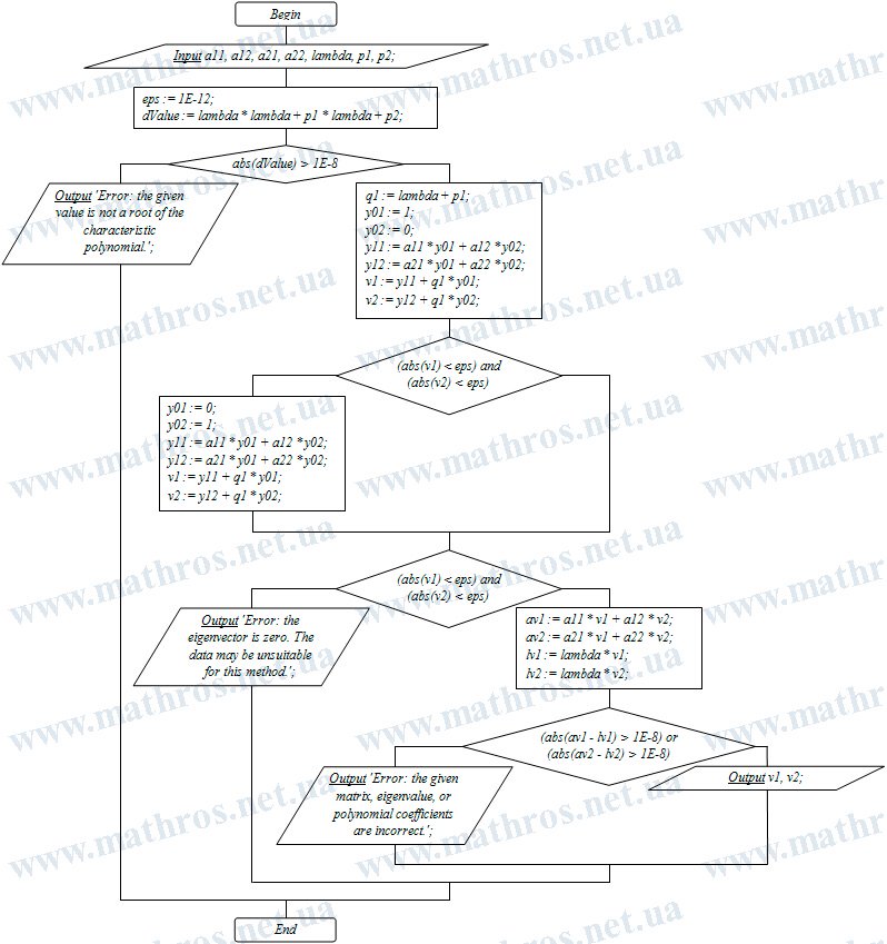
Eigenvectors of a Matrix: Algorithm for Program Implementation
If you enjoy programming, this stage may be the most interesting one. The Krylov method has already given us a clear sequence of actions: construct the Krylov vectors, find the coefficient of the auxiliary polynomial, compute the eigenvector, and check the obtained result.
Now all of this can be turned into a program in any language: Pascal, Python, C++, JavaScript, or any other language you like. Look at the flowchart below and try to implement this algorithm yourself. Isn’t it interesting to see how theoretical formulas turn into real code?