The inverse of a matrix is a concept that appears when we want to do with matrices something similar to what we do with numbers when we divide. We already know how to add and multiply matrices, but what about “division”? In many problems, after multiplying by a matrix \( A \), you need to recover the original vector (or matrix). That’s exactly why it’s important to understand when an inverse matrix exists and how it is found in practice.
Inverse of a Matrix: An Analogy with Numbers and the Exact Definition
Matrices really are similar to numbers in some ways: we can add and multiply them. And in arithmetic, after multiplication, division often comes next. For example, for any nonzero number \( x \), there is a reciprocal number \( \frac{1}{x} \), and the well-known equality holds:
\[
x \cdot \frac{1}{x} = 1.
\]
In matrix algebra, the idea is similar, but there is an important condition. An inverse matrix is defined only for a square matrix \( A \), and not for every square matrix—only for a non-singular one, meaning a matrix for which \( \det(A) \ne 0 \). Why is this so important? Because when \( \det(A)=0 \), the inverse matrix does not exist, and it becomes impossible to obtain the identity matrix through multiplication.
If \( A \) is square and \( \det(A) \ne 0 \), then there exists a matrix \( A^{-1} \), called the inverse of \( A \), and it satisfies:
\[
A \cdot A^{-1} = E,
\]
where \( E \) is the identity matrix. In other words, multiplying \( A^{-1} \) gives the identity matrix, which leaves a matrix of the appropriate size unchanged under multiplication. That is exactly what we expect from an analogue of division.
Inverse of a Matrix: How to Compute It by Solving Linear Systems
We have the definition, but how do you actually compute \( A^{-1} \) in real problems? One of the most convenient approaches is to reduce everything to solving systems of linear equations.
The idea is simple: we solve the matrix equation
\[
A \cdot X = E,
\]
where \( X \) is the unknown matrix we are looking for—namely, \( A^{-1} \).
Next comes a step that makes the whole picture much clearer: we treat \( X \) and \( E \) as collections of column vectors. Let the columns of the matrix \( X \) be
\[
x^{(1)}=\begin{pmatrix}x_{11}\\x_{21}\\x_{31}\\\vdots\\x_{n1}\end{pmatrix},\quad
x^{(2)}=\begin{pmatrix}x_{12}\\x_{22}\\x_{32}\\\vdots\\x_{n2}\end{pmatrix},\quad
x^{(3)}=\begin{pmatrix}x_{13}\\x_{23}\\x_{33}\\\vdots\\x_{n3}\end{pmatrix},\ \ldots,\
x^{(n)}=\begin{pmatrix}x_{1n}\\x_{2n}\\x_{3n}\\\vdots\\x_{nn}\end{pmatrix}.
\]
And let the columns of the identity matrix \( E \) be written as
\[
e^{(1)}=\begin{pmatrix}1\\0\\0\\ \vdots \\0\end{pmatrix},\quad
e^{(2)}=\begin{pmatrix}0\\1\\0\\ \vdots \\0\end{pmatrix},\quad
e^{(3)}=\begin{pmatrix}0\\0\\1\\ \vdots \\0\end{pmatrix},\ \ldots,\
e^{(n)}=\begin{pmatrix}0\\0\\0\\ \vdots \\1\end{pmatrix}.
\]
Then the single matrix equation \( A \cdot X = E \) can be replaced by an equivalent set of independent vector-matrix equations:
\[
A \cdot x^{(1)} = e^{(1)},\quad
A \cdot x^{(2)} = e^{(2)},\quad
A \cdot x^{(3)} = e^{(3)},\ \dots,\
A \cdot x^{(n)} = e^{(n)}.
\]
And here is the key point: all these systems share the same coefficient matrix \( A \). So, if you apply Gaussian elimination, the row transformations (reducing \( A \) to an upper triangular form) are essentially the same for every right-hand side \( e^{(1)}, e^{(2)}, e^{(3)}, \ldots, e^{(n)} \).
You solve the first system and get the first column of the inverse matrix. Then you solve the second system and get the second column, and you continue the same way for all columns. In the end, the vectors \( x^{(1)}, x^{(2)}, x^{(3)}, \ldots, x^{(n)} \) form the matrix \( X \), which is exactly the inverse matrix \( A^{-1} \).
Practical Examples: Step-by-Step Solutions
To make sure this topic doesn’t stay only in theory, let’s move to practice. Below we’ll go through three typical situations: when the inverse of a matrix does not exist, when it does exist and can be found, and when the very setup of the problem already tells you that inversion is impossible. Pay attention not only to the final answer, but also to the logic of the checks—this can save you a lot of time.
Example 1. Find the inverse of a matrix
\[
A=\begin{pmatrix}
2 & -1 & 4\\
4 & -2 & 8\\
6 & -3 & 12
\end{pmatrix}.
\]
First, let’s check the conditions for the inverse of a matrix to exist. The matrix \( A \) is square (size \( 3\times 3 \)), so the first condition is satisfied. Now we check the second condition—whether \( \det(A)\ne 0 \).
Here it is convenient to notice that the second row equals the first row multiplied by \( 2 \), and the third row equals the first row multiplied by \( 3 \). That means the rows are linearly dependent, so
\[
\det(A)=0.
\]
So the matrix \( A \) is singular, and therefore the inverse matrix \( A^{-1} \) does not exist.
Example 2. Find the inverse of a matrix
\[
A=\begin{pmatrix}
5 & -6 & 7 & 1\\
7 & 10 & -9 & 8\\
3 & 3 & 5 & 1\\
-10 & 2 & 3 & 4
\end{pmatrix}.
\]
First, we check the conditions for the inverse of a matrix to exist. Since the given matrix \( A \) is square (size \( 4\times 4 \)), the first condition holds. Now we check the second condition, meaning we find out whether the determinant of \( A \) is nonzero:
\[
\det(A)=
\begin{vmatrix}
5 & -6 & 7 & 1\\
7 & 10 & -9 & 8\\
3 & 3 & 5 & 1\\
-10 & 2 & 3 & 4
\end{vmatrix}.
\]
Expanding the determinant along the first row, we get:
\[
\det(A)=
5 \cdot \begin{vmatrix}
10 & -9 & 8\\
3 & 5 & 1\\
2 & 3 & 4
\end{vmatrix}
+6 \cdot \begin{vmatrix}
7 & -9 & 8\\
3 & 5 & 1\\
-10 & 3 & 4
\end{vmatrix}
+7 \cdot \begin{vmatrix}
7 & 10 & 8\\
3 & 3 & 1\\
-10 & 2 & 4
\end{vmatrix}
-1 \cdot \begin{vmatrix}
7 & 10 & -9\\
3 & 3 & 5\\
-10 & 2 & 3
\end{vmatrix}.
\]
After calculations, we obtain:
\[
\det(A) = 5\cdot 252 + 6\cdot 789 + 7\cdot 138 – 1\cdot(-921) = 7881 \neq 0.
\]
So the matrix \( A \) is square and non-singular, which means the inverse matrix \( A^{-1} \) exists. Now we move on to computing it and apply the approach based on the equation \( A \cdot X=E \).
Since \( E \) is the identity matrix of order \( 4 \), we get four independent systems of linear equations:
\[
\begin{array}{cc}
\begin{cases}
5\cdot x_1-6\cdot x_2+7\cdot x_3+1\cdot x_4=1\\
7\cdot x_1+10\cdot x_2-9\cdot x_3+8\cdot x_4=0\\
3\cdot x_1+3\cdot x_2+5\cdot x_3+1\cdot x_4=0\\
-10\cdot x_1+2\cdot x_2+3\cdot x_3+4\cdot x_4=0
\end{cases},
&
\begin{cases}
5\cdot x_1-6\cdot x_2+7\cdot x_3+1\cdot x_4=0\\
7\cdot x_1+10\cdot x_2-9\cdot x_3+8\cdot x_4=1\\
3\cdot x_1+3\cdot x_2+5\cdot x_3+1\cdot x_4=0\\
-10\cdot x_1+2\cdot x_2+3\cdot x_3+4\cdot x_4=0
\end{cases},
\\[6pt]
\begin{cases}
5\cdot x_1-6\cdot x_2+7\cdot x_3+1\cdot x_4=0\\
7\cdot x_1+10\cdot x_2-9\cdot x_3+8\cdot x_4=0\\
3\cdot x_1+3\cdot x_2+5\cdot x_3+1\cdot x_4=1\\
-10\cdot x_1+2\cdot x_2+3\cdot x_3+4\cdot x_4=0
\end{cases},
&
\begin{cases}
5\cdot x_1-6\cdot x_2+7\cdot x_3+1\cdot x_4=0\\
7\cdot x_1+10\cdot x_2-9\cdot x_3+8\cdot x_4=0\\
3\cdot x_1+3\cdot x_2+5\cdot x_3+1\cdot x_4=0\\
-10\cdot x_1+2\cdot x_2+3\cdot x_3+4\cdot x_4=1
\end{cases}.
\end{array}
\]
After the forward step of Gaussian elimination, each system is reduced to triangular form:
\[
\begin{array}{cc}
\begin{cases}
x_1-1.2\cdot x_2+1.4\cdot x_3+0.2\cdot x_4=0.2\\
x_2-1.022\cdot x_3+0.359\cdot x_4=-0.076\\
x_3-0.261\cdot x_4=-0.013\\
x_4=0.117
\end{cases},
&
\begin{cases}
x_1-1.2\cdot x_2+1.4\cdot x_3+0.2\cdot x_4=0\\
x_2-1.022\cdot x_3+0.359\cdot x_4=0.054\\
x_3-0.261\cdot x_4=-0.047\\
x_4=0.076
\end{cases},
\\[6pt]
\begin{cases}
x_1-1.2\cdot x_2+1.4\cdot x_3+0.2\cdot x_4=0\\
x_2-1.022\cdot x_3+0.359\cdot x_4=0\\
x_3-0.261\cdot x_4=1.113\\
x_4=-0.079
\end{cases},
&
\begin{cases}
x_1-1.2\cdot x_2+1.4\cdot x_3+0.2\cdot x_4=0\\
x_2-1.022\cdot x_3+0.359\cdot x_4=0\\
x_3-0.261\cdot x_4=0\\
x_4=0.088
\end{cases}.
\end{array}
\]
Next we perform back substitution and obtain the columns of \( A^{-1} \):
\[
x^{(1)}=\begin{pmatrix}0.032\\-0.100\\0.018\\0.117\end{pmatrix},\quad
x^{(2)}=\begin{pmatrix}0.022\\-0.001\\-0.027\\0.076\end{pmatrix},\quad
x^{(3)}=\begin{pmatrix}0.029\\0.142\\0.112\\-0.079\end{pmatrix},\quad
x^{(4)}=\begin{pmatrix}-0.060\\-0.008\\0.023\\0.088\end{pmatrix}.
\]
Therefore,
\[
A^{-1}=
\begin{pmatrix}
0.032 & 0.022 & 0.029 & -0.060\\
-0.100 & -0.001 & 0.142 & -0.008\\
0.018 & -0.027 & 0.112 & 0.023\\
0.117 & 0.076 & -0.079 & 0.088
\end{pmatrix}.
\]
Example 3. Find the inverse of a matrix
\[
A=\begin{pmatrix}
0 & -1 & 3 & 0 & 2\\
2 & -4 & 1 & 5 & 3\\
-4 & 5 & 7 & -10 & 0\\
-2 & 1 & 8 & -5 & 3
\end{pmatrix}.
\]
First, let’s check the conditions for the inverse matrix to exist. Here we immediately see that the matrix has size \( 4\times 5 \), so it is not square. And an inverse matrix is defined only for square matrices.
So for this matrix \( A \) the matrix \( A^{-1} \) does not exist already by the first condition.
What to Learn Next: Useful Topics to Keep Going
If you enjoyed working with inverse matrices, it makes sense to take the next step and expand into related topics. Where should you start? Below are three directions that naturally build on the inverse of a matrix idea and give you new tools for solving problems.
- Inverse of a Matrix Using the Gauss–Jordan Method: A Fast Practical Algorithm — We’ll go through a step-by-step transformation scheme that helps you find an inverse matrix through an augmented matrix quickly and confidently.
- Inverse of a Matrix via Cofactors: The Logic of Minors and Determinants — We’ll explain how cofactors work and how they lead to the classical construction of the inverse matrix.
- Inverse of a Matrix and the Characteristic Polynomial: An Unusual but Powerful Approach — We’ll show how the coefficients of the characteristic polynomial can help you obtain an inverse matrix when you need theory at a more serious level.
Inverse of a Matrix and Programming: Turn a Flowchart into Code
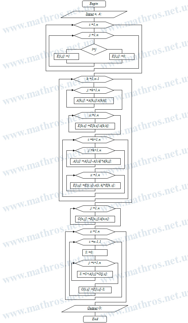
If you’re interested in programming, a ready-made flowchart can be a great starting point for a small project: a program that computes the inverse of a matrix by solving the corresponding systems of linear equations. Carefully follow the diagram from the input data to the final result, and think about how each block can be expressed as a few clear lines of code. Isn’t it satisfying when, after you run your program, the matrix \( A^{-1} \) appears automatically—rather than after a long series of manual calculations?
This kind of practice strengthens two skills at once: it helps you truly understand the mathematics, and it trains you to translate an algorithm from a diagram into a working solution.