The determinant of a matrix is a fundamental concept in linear algebra that every student in technical or mathematical fields will encounter sooner or later. It is more than just a number next to a matrix; it is an important characteristic that describes the properties of the matrix itself and the linear transformations related to it.
With the determinant of a matrix, you can solve systems of linear equations, check if a system has a unique solution, and find eigenvalues and eigenvectors. Additionally, determinants are used in systems theory, probability theory, physics, engineering, and numerical methods. Isn’t it convenient when one number can provide so much information about a problem?
In this article, we will go step by step to explain what the determinant of a matrix is, its key properties, and how to calculate it for matrices of different sizes. We will also discuss its geometric meaning and explore simple examples, ensuring that theory is connected to real-life problems and is easy to understand.
Basic Concept: What Is the Determinant of a Square Matrix?
Let’s start with the basics. The determinant of a square matrix is a numerical characteristic that corresponds to every square matrix. For a matrix \(A\), the determinant is usually written as \(\det(A)\) or \(|A|\). Sometimes, the symbol \(\Delta\) is also used.
Why are we talking specifically about square matrices? Because the determinant is only defined for them. While rectangular matrices are useful, they do not have their own determinant.
How should we think about this number? In general, it is calculated using special formulas that consider the matrix’s elements and their arrangement in rows and columns. From the definition, we can see that the determinant is “sensitive” to the structure of the matrix, not just the numbers it contains.
Applications: Where the Determinant of a Matrix is Used in Practice
What does this number offer in practice? First, the determinant is closely related to the existence of the inverse matrix. If \(\text{det}(A) \neq 0\), the matrix \(A\) has an inverse matrix \(A^{-1}\). Conversely, if the determinant is zero, the inverse matrix does not exist. This is a very important criterion that is often used in theory and practical problems.
Second, the determinant helps to analyze systems of linear equations. For example, with a system that has a square coefficient matrix:
- If \(\text{det}(A) \neq 0\), the system has a unique solution.
- If\(\text{det}(A) = 0\), the system either has an infinite number of solutions or is inconsistent.
Additionally, determinants show up in formulas for eigenvalues and eigenvectors, in various physical laws, and in probability theory and statistics. Therefore, studying determinants is not just a “formality” but an important tool that continues to appear in other topics.
Properties: Key Rules for the Determinant of a Matrix
To work confidently with determinants, it’s important to know their properties. These properties help simplify calculations and allow us to draw conclusions about the matrix quickly, even before performing detailed computations. Let’s go over the main ones.
- Swapping Rows or Columns: If two rows (or two columns) of a matrix are swapped, the sign of the determinant changes to the opposite.
- Non-zero Determinant and the Inverse Matrix: If matrix \(A\) has a non-zero determinant, then it has an inverse matrix \(A^{-1}\), and \(\text{det}(A^{-1}) = \frac{1}{\text{det}(A)}\).
- Zero Row or Column: If any row (or column) of a matrix consists entirely of zeros, the determinant of that matrix is zero.
- Identical Rows or Columns: If two rows (or two columns) of a matrix are identical, its determinant is also zero.
- Linear Combination of Rows or Columns: If one row (or column) is a linear combination of others, the determinant is zero. This is due to the linear dependence of the corresponding vectors.
- Identity Matrix and Diagonal Matrices: If a matrix has ones on the main diagonal and zeros elsewhere (an identity matrix), then \(\text{det}(A) = 1\).
- Adding a Multiple of Another Row or Column: If one row (or column) is replaced by itself plus a constant multiple of another row (or column), the determinant does not change. This property is especially useful in matrix transformations.
- Triangular Matrices: If a matrix is upper or lower triangular, its determinant is the product of the elements on the main diagonal: \(\text{det}(A) = a_{11} \cdot a_{22} \cdot a_{33} \cdot \dots \cdot a_{nn}\).
- Matrix Multiplication: For two square matrices of the same size, \(\text{det}(A \cdot B) = \text{det}(A) \cdot \text{det}(B)\).
- Transposition: The determinant of a transposed matrix does not change: \(\text{det}(A^T) = \text{det}(A)\).
These properties often help us quickly determine whether the determinant will be zero or simplify the matrix into a more convenient form, without needing to perform the full calculation.
Simple Cases: Formulas for the Determinant of a 2×2 and 3×3 Matrix
Before moving on to more complex cases, it’s helpful to review how the determinant is calculated for the simplest matrices — those of size 2×2 and 3×3.
2×2 Matrix — A Simple Start
Consider the matrix
\[
A =
\begin{pmatrix}
a_{11} & a_{12} \\
a_{21} & a_{22}
\end{pmatrix};
\]
The determinant is calculated using the following formula:
\[
\det(A) =
\begin{vmatrix}
a_{11} & a_{12} \\
a_{21} & a_{22}
\end{vmatrix}
= a_{11} \cdot a_{22} – a_{12} \cdot a_{21}
\tag{1}
\]
In this case, you multiply the elements of the main diagonal, then multiply the elements of the off-diagonal, and subtract the second product from the first. It’s simple and easy to remember.
3×3 Matrix — Sarrus’ Rule (The Triangle Rule)
For a 3×3 matrix
\[
A =
\begin{pmatrix}
a_{11} & a_{12} & a_{13} \\
a_{21} & a_{22} & a_{23} \\
a_{31} & a_{32} & a_{33}
\end{pmatrix};
\]
we often use Sarrus’ Rule (also known as the “triangle rule”).
The method is as follows: first, take the sum of the three products of the elements going “down and to the right” (along the main diagonal and the two diagonals parallel to it). Then, subtract the sum of the three products of the elements going “down and to the left” (along the side diagonal and the two diagonals parallel to it). The formula is:
\[
\det(A) =
\begin{vmatrix}
a_{11} & a_{12} & a_{13} \\
a_{21} & a_{22} & a_{23} \\
a_{31} & a_{32} & a_{33}
\end{vmatrix}
= a_{11} \cdot a_{22} \cdot a_{33}
+ a_{12} \cdot a_{23} \cdot a_{31}
+ a_{13} \cdot a_{21} \cdot a_{32}
– a_{13} \cdot a_{22} \cdot a_{31}
– a_{11} \cdot a_{23} \cdot a_{32}
– a_{12} \cdot a_{21} \cdot a_{33}
\tag{2}
\]
This rule is useful for manual calculations and shows how elements from different rows and columns combine in the determinant.
The Minor Method: Calculating the Determinant of Higher-Order Matrices
When the size of a matrix exceeds 3×3, simple “ready-made” formulas are no longer available. However, there is a general approach that works for matrices of any order. This approach relies on the concepts of minors and cofactors.
Minor and Cofactor — Two Key Concepts
Let’s consider a square matrix of order \(n\). Then:
- The minor \(M_{ij}\) of an element \(a_{ij}\) is the determinant of the matrix of order \(n-1\), obtained by deleting the \(i\)-th row and the \(j\)-th column from the original matrix.
- The cofactor \(A_{ij}\) of an element \(a_{ij}\) is the minor with a “sign” that depends on the sum of the indices:
\[
A_{ij} = (-1)^{i+j} \cdot M_{ij};
\]
Thus, each element of the matrix is “linked” to its minor and cofactor.
Expansion by Row or Column
Using cofactors, the determinant of matrix \(A\) can be calculated by expanding it along any row or column. For example, if we expand along the \(i\)-th row, we get:
\[
\det(A) = a_{i1} \cdot A_{i1} + a_{i2} \cdot A_{i2} + a_{i3} \cdot A_{i3} + \dots + a_{in} \cdot A_{in}
\tag{3}
\]
In this case, we multiply each element of the chosen row by its cofactor and sum all these products. Similarly, we can expand along any column.
In practice, this approach is often applied recursively: to compute the determinant of a matrix of order \(n\), we first compute several determinants of order \(n-1\). For those, we apply the expansion again, continuing until we reach 2×2 or 3×3 matrices, where formulas (1) and (2) can be used.
Practical Tip — How to Choose a Row or Column
Can you choose any row or column for the expansion? Yes, the result will be the same. However, from a computational perspective, it’s better to choose a row or column with the most zero elements. This way, some terms in formula (3) will immediately be zero, and fewer minors will need to be computed.
This approach is especially useful in programming: choosing the right row or column can significantly reduce the number of operations.
Geometry: The Geometric Meaning of the Determinant of a Matrix
It is important to discuss the geometric meaning of the determinant separately. It helps us better understand what this number actually “measures”.
2×2 Case — Area of a Parallelogram
Consider the matrix
\[
A =
\begin{pmatrix}
a_{11} & a_{12} \\
a_{21} & a_{22}
\end{pmatrix};
\]
Its columns can be viewed as vectors in the plane:
- The first vector goes from the point \((0,0)\) to \((a_{11}, a_{21})\).
- The second vector goes from the point \((0,0)\) to \((a_{12}, a_{22})\).
These two vectors form a parallelogram.

The absolute value of the determinant of matrix \(A\) equals the area of this parallelogram:
\[
S = \left| a_{11} \cdot a_{22} – a_{12} \cdot a_{21} \right|.
\]
Furthermore, the sign of the determinant indicates the “orientation” of the vector pair: whether we “turn” from the first vector to the second in a clockwise or counterclockwise direction. If the determinant is positive, the orientation is one way; if negative, it is the opposite. If the determinant is zero, the vectors lie on the same line, meaning the parallelogram has “collapsed”, and its area is zero.
Higher Dimensions — Volume of a Parallelepiped and \(n\)-Dimensional Volumes
In three-dimensional space (for a 3×3 matrix), the geometric meaning of the determinant is related to the volume of the parallelepiped formed by the column vectors of the matrix. For an n×n matrix, the determinant can be interpreted as the “volume” of an \(n\)-dimensional parallelepiped. This is harder to visualize, but the concept remains the same: the determinant shows how the matrix “stretches” or “compresses” a unit volume in the corresponding space.
Practice with Determinants: Examples and Explanations
To ensure the topic is not just theoretical, let’s move on to some practical problems. Step by step, we will solve a few typical examples of calculating the determinant of a matrix and apply the properties you’ve already learned. Pay attention not only to the answer but also to the logic behind it — this logic helps you quickly navigate similar exercises.
Example 1: What is the determinant of a matrix \(A\) if all its elements are zero?
Let’s recall the property: if all the elements of at least one row (or column) are zero, the determinant of such a matrix is zero. Here, all rows consist of zeros, so this condition is definitely satisfied.
Thus,
\[
\det(A) = 0;
\]
Example 2: What is the determinant of a matrix \(A\) if all its elements are the same?
In this case, all the elements of matrix \(A\) are identical, for example, equal to some number \(c\). What does this mean for the rows and columns?
In such a matrix, all the rows are identical (and similarly, all the columns are identical). We already know an important property: if a matrix has at least two identical rows or columns, its determinant equals zero.
Thus, regardless of the size of the matrix, we have:
\[
\det(A) = 0;
\]
Example 3: Calculate the determinant of a 2×2 matrix
\[
A =
\begin{pmatrix}
1 & 5 \\
3 & 1
\end{pmatrix};
\]
Using the formula for a 2×2 matrix:
\[
\det(A) =
\begin{vmatrix}
1 & 5 \\
3 & 1
\end{vmatrix}
= 1 \cdot 1 – 5 \cdot 3 = 1 – 15 = -14;
\]
Thus, the determinant of matrix \(A\) is \(-14\).
Example 4: Calculate the determinant of a 3×3 matrix
\[
A =
\begin{pmatrix}
2 & 4 & 5 \\
1 & 0 & 3 \\
3 & -1 & 2
\end{pmatrix};
\]
We’ll use Sarrus’ rule (the triangle rule). Then:
\[
\det(A) =
\left|
\begin{matrix}
2 & 4 & 5 \\
1 & 0 & 3 \\
3 & -1 & 2
\end{matrix}
\right|
= 2 \cdot 0 \cdot 2 + 4 \cdot 3 \cdot 3 + 5 \cdot 1 \cdot (-1)
– 5 \cdot 0 \cdot 3 – 4 \cdot 1 \cdot 2 – 2 \cdot 3 \cdot (-1);
\]
Now, let’s calculate step by step:
\[
\det(A) = 0 + 36 – 5 – 0 – 8 + 6 = 29;
\]
Thus, the determinant of matrix \(A\) is \(29\).
Example 5: Calculate the determinant of a 4×4 matrix
\[
A =
\begin{pmatrix}
1 & 5 & 3 & -4 \\
3 & 1 & -2 & 0 \\
5 & -7 & 0 & 10 \\
0 & 3 & -5 & 0
\end{pmatrix};
\]
Notice the last (fourth) row: it contains two zeros. This is useful because expanding along this row will allow us to calculate the determinant with fewer computations. So, let’s expand along the fourth row:
\[
\det(A) = a_{41} \cdot A_{41} + a_{42} \cdot A_{42} + a_{43} \cdot A_{43} + a_{44} \cdot A_{44};
\]
For the elements of the fourth row, we have:
\[
a_{41} = 0;\quad a_{42} = 3;\quad a_{43} = -5;\quad a_{44} = 0;
\]
So, the formula now contains only non-zero terms:
\[
\det(A) = 3 \cdot A_{42} – 5 \cdot A_{43};
\]
Now, let’s find the corresponding cofactors:
\[
A_{42} = (-1)^{4+2} \cdot
\left|
\begin{matrix}
1 & 3 & -4 \\
3 & -2 & 0 \\
5 & 0 & 10
\end{matrix}
\right|
= (-1)^6 \cdot (-150) = -150;
\]
\[
A_{43} = (-1)^{4+3} \cdot
\left|
\begin{matrix}
1 & 5 & -4 \\
3 & 1 & 0 \\
5 & -7 & 10
\end{matrix}
\right|
= (-1)^7 \cdot (-36) = 36;
\]
Substituting these values into the expansion formula:
\[
\det(A) = 3 \cdot (-150) – 5 \cdot 36 = -450 – 180 = -630;
\]
Thus, the determinant of matrix \(A\) is \(-630\).
What to Study Next: Useful Topics for Further Exploration
If you enjoyed working with determinants, it’s a good idea to take the next step and explore related topics. Where should you begin?
- Inverse Matrix and Determinant: When a Matrix Has an Inverse — You’ll see how a non-zero determinant guarantees the existence of an inverse matrix and plays a role in formulas for finding it.
- Gaussian Elimination and the Determinant: The Path to Triangular Form — You will learn how to transform a matrix into triangular form and find the determinant as the product of the diagonal elements.
- Systems of Equations and Determinants: Cramer’s Rule in Practice — You will learn how to solve small systems of equations using Cramer’s rule and how determinants appear in the formulas.
These topics build on each other and will help you gain a deeper understanding of how determinants are used in various areas of linear algebra and its applications.
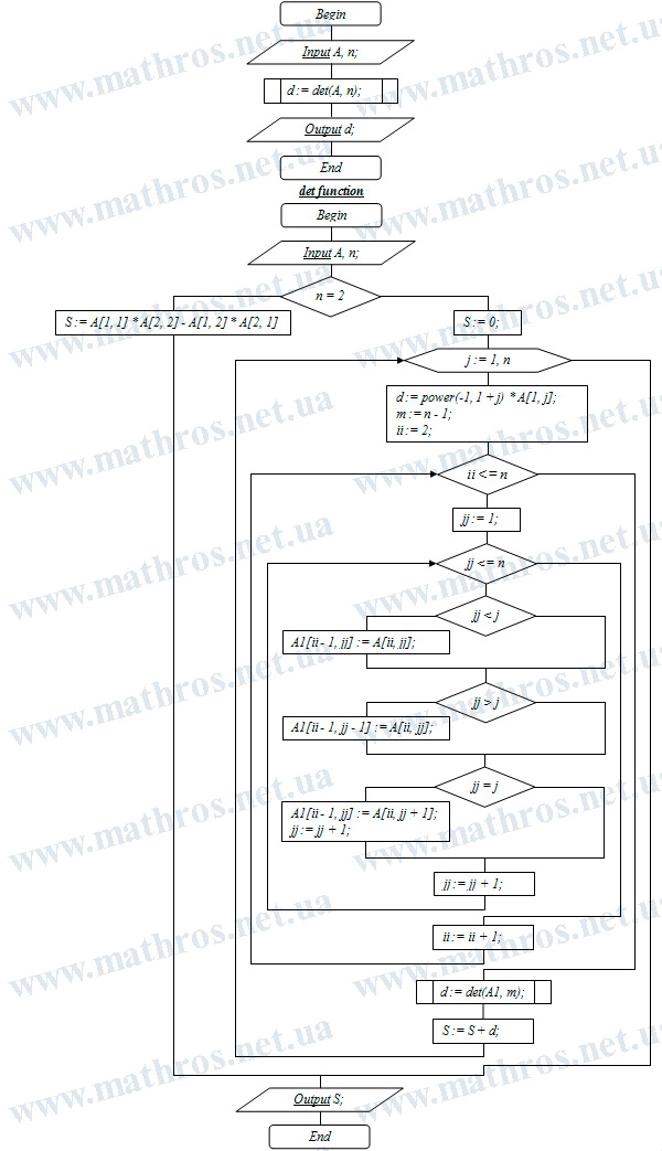
Determinant of a Matrix: A Flowchart as the Basis for Code
If you’re interested in programming, the flowchart of the algorithm for expanding a determinant along the first row could serve as the foundation for a simple program in your preferred language. Look at the diagram and follow the process: from the input matrix to the resulting determinant value. Then imagine that each block represents a few lines of code. This way, you can transfer the algorithm into Python, C++, Java, or any other language, and compute determinants of matrices of various sizes with a single run of the program. This exercise will help you better understand the “Determinant of a Matrix” topic and practice turning flowcharts into working code.