Milne’s method is a powerful technique for anyone aiming to confidently solve differential equations. If you are familiar with numerical methods, you already know that they help us find approximate solutions when analytical methods become too complex or even impossible. However, Milne’s method stands out due to its unique logic and efficiency. In this article, we’ll dive into how Milne’s method works, explore why its “predict-correct” approach leads to great accuracy, and show you how to apply it with minimal effort. Not only will you gain a solid understanding of the theory behind it, but you’ll also see how this method is used in practice to solve specific problems.
What is Milne’s Method and Why is It So Popular?
Milne’s method is a convenient and quite accurate way to approximate solutions to the Cauchy problem for ordinary differential equations. It is part of the multistep methods, which means that each step uses several previous calculations to refine the result. Does it sound complicated? It’s actually quite the opposite! Students and researchers frequently use this method because it’s simple to implement.
So, what makes Milne’s method stand out? The key is its “predict-correct” scheme. First, we make a prediction of the function’s value at a new point using the known values from previous steps. Then, we check the accuracy of the prediction and adjust it if needed. This two-step strategy enables Milne’s method to achieve better accuracy than simpler methods.
How to Apply Milne’s Method to a Cauchy Problem: Where to Start?
Let’s consider a standard Cauchy problem:
![]()
Here’s what we need to do: First, we choose the integration step h=[b-a]/n, and then we create a grid of points:
![]()
But there’s one important catch: to compute yi+1 using Milne’s method, we need the values from the previous four steps. Where do we get these values from? Initially, we use one of the single-step methods—such as Euler’s or Runge-Kutta’s methods. These methods help us calculate the first four values: y0, y1, y2, y3, and then Milne’s method takes over.
Step-by-Step Milne’s Algorithm: Predict → Correct
Once we have the first four points, we can proceed to calculate the next values (starting from i=4). The process is simple: first, predict, then correct. In the prediction step, we estimate the new point based on the previous derivatives y’i-2, y’i-1, y’i. We get the predicted value:
![]()
Next, we substitute ỹi+1 into the equation to find ỹ’i+1=f(xi+1, ỹi+1). After that, we make the correction, which “smooths” the prediction between the neighboring nodes:
![]()
Do we need to repeat the correction? Sometimes yes, but typically one round of “predict → correct” is sufficient. We continue using the same pattern, calculating each step, and gradually build the solution for the entire interval.
Why These Formulas?
The idea is straightforward: we approximate the derivative y’=f(x,y) using Newton’s interpolation polynomial on a uniform grid, and then integrate this polynomial over the corresponding interval. For the prediction step, we use a third-order polynomial at the nodes xi-3, xi-2, xi-1, xi:
![]()
Next, we approximate the integral of the derivative by integrating P3(x):
![]()
Integrating the polynomial terms over the interval [xi-3, xi+1] gives the prediction formula:
![]()
For correction, we use a second-order polynomial at the nodes xi-1, xi, xi+1:
![]()
After integrating P2(x) over the interval [xi-1, xi+1], we get the corrector:
![]()
Here, in practice, the unknown y’i+1 is replaced with the approximate value ỹ’i+1=f(xi+1, ỹi+1). Thus, the formulas naturally emerge from interpolating y’ on the grid and then integrating over the required segment.
The Advantage of Milne’s Method: More Data Equals a More Accurate Result
Unlike single-step methods, Milne’s method uses data from four previous points. This allows for a more accurate prediction of the next value, as it incorporates more data from the history of calculations. Additionally, the correction step helps control the error and adjust it when necessary by aligning the result with neighboring nodes. As a result, you obtain more stable values with better accuracy without significantly increasing computational effort. So, more data at the input leads to more reliable results at the output.
Applying Milne’s Method in Practice: A Step-by-Step Example
Now that we’ve covered the theory, let’s see Milne’s method in action. Reading through the formulas is one thing, but actually working through a concrete example gives you a much clearer understanding of how convenient and effective this method is.
Example 1: We Have the Differential Equation y’=y-x with the Initial Condition y(0)=1.5. We Need to Find the Approximate solution to This Equation on the Interval [0, 1] and Compare the Results with the Exact Solution, Which is y(x)=0.5⋅ex+x+1
First, let’s divide the interval [0, 1] into 8 equal parts, so the integration step is h=0.125. The nodes will be as follows:
![]()
Since Milne’s method is multistep, we need the first four values: y0, y1, y2, y3.
To save time, we use an online Runge-Kutta fourth-order method calculator to quickly and accurately get these initial points. We input the equation y’=y-x, the initial condition y(0)=1.5, the exact solution, the interval [0, 1] and the number of parts n=8. The result gives us:
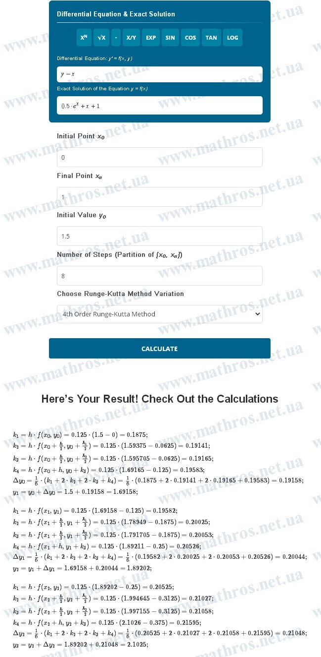
These values are now our starting points for Milne’s method.
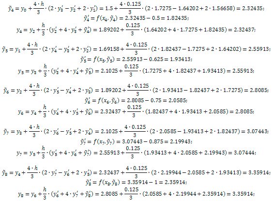
Next, using the prediction and correction formulas, we proceed step by step to calculate the next values:
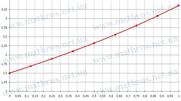
Now, let’s compare the results with the exact values:
| x | Approximate y | Exact y | Error |
|---|---|---|---|
| 0.5 | 2.32437 | 2.32436 | 0.00001 |
| 0.625 | 2.55913 | 2.55912 | 0.00001 |
| 0.75 | 2.8085 | 2.8085 | 0 |
| 0.875 | 3.07444 | 3.07444 | 0 |
| 1 | 3.35914 | 3.35914 | 0 |
As we can see, the results are nearly perfect. The errors are either minimal or completely absent after just 8 steps.
Milne’s method is not just another formula from a textbook. It’s a powerful tool that delivers highly accurate results with minimal effort, especially when combined with methods like Runge-Kutta to set the initial values. Theory and practice work together beautifully here.
Want to Learn More? Other Interesting Numerical Methods for Solving Differential Equations
Milne’s method is undoubtedly one of the most effective ways to numerically solve differential equations. However, it’s not the only one. There are many other methods in numerical analysis that are just as useful and effective. If you’re interested and want to expand your knowledge, consider these methods:
- Adams’ Method – Another multistep approach that uses several previous data points to improve accuracy, allowing for more reliable predictions and reduced errors.
- Modified Euler’s Method – An improved version of the classic Euler method. It averages the derivative between points for better accuracy without significantly increasing computational costs.
- Runge-Kutta-Merson Method – One of the most accurate methods, automatically controlling precision by adjusting the integration step. This makes it particularly useful for problems where minimizing error accumulation is essential.
Each of these methods has its strengths and applications. By exploring them, you’ll be able to choose the right tool for any problem you encounter. In numerical analysis, there is no single “perfect” method—only the one that best fits your particular needs.
Bring Mathematics to Code: Create Your Own Solution
Mastering Milne’s method allows you to solve complex problems not just on paper, but in your own programs. Imagine how much more efficient it would be to automate calculations, so you don’t have to perform dozens of manual steps. Let your computer do the heavy lifting!
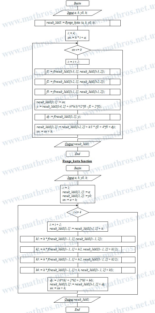
You can use any programming language you’re comfortable with—Python, Java, C++, or even JavaScript. The key is that the process should be clear and fun for you. Below is a flowchart illustrating Milne’s method algorithm step by step. It will help you quickly understand the logic behind the calculations and transfer it into code. Use it as a guide, adapt it to your needs, and create a program that will be your personal tool for precise and fast calculations.