The power rule is one of the main rules of differential calculus. It is used when we need to find the derivative of a power function. Most often, it applies to functions where a variable is raised to a constant numerical power. That is why this rule appears so often when differentiating polynomials, rational expressions, and functions written using powers.
At first glance, it may seem that it is enough just to memorize this rule. But is that approach always enough? Not really. To apply the formula confidently, it is important to understand where it comes from. Then the power rule is not seen as a mechanical action, but as a logical result of the definition of the derivative.
Power Rule: The Main Formula for a Power Function
Suppose we have a power function
\[
y=x^n,
\]
where \( n \) is a constant numerical exponent. Then the derivative of this function is found using the formula
\[
y’=n\cdot x^{n-1}.
\]
This is the main formula of the power rule. It is also often written using the differentiation operator:
\[
\frac{d}{dx}\left(x^n\right)=n\cdot x^{n-1}.
\]
Both forms mean the same thing. The first form is convenient when the function is denoted by \( y \). The second form is used more often in a general setting, when we want to show directly that we are taking the derivative of the expression \( x^n \).
So, the rule works like this: the exponent \( n \) moves in front of the variable as a multiplier, and the exponent itself decreases by one. For example, for the function \( y=x^5 \), we get the derivative \( y’=5\cdot x^4 \). And for the function \( y=x^2 \), we get \( y’=2\cdot x \).
However, it is important not only to know the ready-made formula. Why exactly does the exponent become a multiplier? And why is the new exponent equal to \( n-1 \)? To answer these questions, let’s look at the derivation of the formula using the definition of the derivative.
Step by Step: Deriving the Formula Using the Definition of the Derivative
Now let’s look carefully at where the power rule formula comes from. To do this, we will use the definition of the derivative using a limit. Suppose the function is given as
\[
y=x^n.
\]
By the definition of the derivative, we have
\[
y’=\lim_{h\to 0}\frac{y(x+h)-y(x)}{h}.
\]
Since \( y(x)=x^n \), the value of this function at the point \( x+h \) is
\[
y(x+h)=(x+h)^n.
\]
Now substitute these expressions into the definition of the derivative:
\[
y’=\lim_{h\to 0}\frac{(x+h)^n-x^n}{h}.
\]
At this stage, we have obtained the correct expression for the derivative, but it does not yet look like the power rule formula. What should we do next? We need to expand the power \( (x+h)^n \). For a natural number \( n \), this is conveniently done using the binomial theorem:
\[
(x+h)^n=x^n+n\cdot x^{n-1}\cdot h+\frac{n\cdot (n-1)}{2}\cdot x^{n-2}\cdot h^2+\ldots+h^n.
\]
Now substitute this expansion into the derivative formula:
\[
y’=\lim_{h\to 0}
\frac{
x^n+n\cdot x^{n-1}\cdot h+\frac{n\cdot (n-1)}{2}\cdot x^{n-2}\cdot h^2+\ldots+h^n-x^n
}{h}.
\]
In the numerator, there are two opposite terms: \( x^n \) and \( -x^n \). They cancel each other out. Therefore, we get
\[
y’=\lim_{h\to 0}
\frac{
n\cdot x^{n-1}\cdot h+\frac{n\cdot (n-1)}{2}\cdot x^{n-2}\cdot h^2+\ldots+h^n
}{h}.
\]
Now let’s pay attention to one common feature of all the terms in the numerator. Each of them contains the factor \( h \). That is why all terms in the numerator can be divided by \( h \). After simplifying, we have
\[
y’=\lim_{h\to 0}
\left(
n\cdot x^{n-1}
+
\frac{n\cdot (n-1)}{2}\cdot x^{n-2}\cdot h
+
\ldots
+
h^{n-1}
\right).
\]
Now the expression has become much simpler. The first term, \( n\cdot x^{n-1} \), no longer contains \( h \). All the other terms contain \( h \), \( h^2 \), \( h^3 \), and so on. Therefore, when \( h\to 0 \), these terms approach zero.
So, after taking the limit, only the first term \( n\cdot x^{n-1} \) remains. Therefore, we finally get
\[
\frac{d}{dx}\left(x^n\right)=n\cdot x^{n-1}.
\]
Thus, the power rule follows directly from the definition of the derivative using a limit. The main step in the derivation is to expand \( (x+h)^n \), cancel the identical terms, and see that after division by \( h \), all terms that contain \( h \) approach zero when taking the limit. That is exactly why the multiplier \( n \) appears in the final formula, and the exponent decreases by one.
Power Rule: Practical Use of the Formula
After the theoretical explanation, it is worth moving on to practice. Examples clearly show how the power rule works and why it makes finding derivatives much simpler. In addition, practical calculations help you remember the formula better and apply it more confidently when differentiating.
Example 1. Find the derivative of the function \( y=x^6 \)
In this example, we have a simple power function. The variable \( x \) is raised to the sixth power, so the exponent is \( 6 \).
According to the power rule, the exponent moves in front of the variable as a multiplier, and the exponent itself decreases by one. Therefore, we have:
\[
y’=\left(x^6\right)’=6\cdot x^{6-1}.
\]
Now let’s calculate the new exponent:
\[
6-1=5.
\]
So,
\[
y’=6\cdot x^5.
\]
Example 2. Find the derivative of the function \( y=4\cdot x^5 \)
Here, the power function has a numerical coefficient. The number \( 4 \) appears before the expression \( x^5 \). What should we do with it? We do not need to change it, because a constant multiplier remains in front of the derivative.
Let’s factor out the constant multiplier \( 4 \) and apply the power rule to \( x^5 \):
\[
y’=4\cdot \left(x^5\right)’.
\]
Since
\[
\left(x^5\right)’=5\cdot x^4,
\]
we get:
\[
y’=4\cdot 5\cdot x^4=20\cdot x^4.
\]
Here, it is important not to forget about the coefficient \( 4 \). It does not disappear. Instead, it is multiplied by the result of differentiating the power part.
Example 3. Find the derivative of the function \( y=\frac{1}{x^3} \)
In this example, the function is written as a fraction. However, it is convenient to rewrite it using a negative exponent. This way, we can apply the power rule directly.
Let’s rewrite the given function in power form:
\[
y=x^{-3}.
\]
Now we can see that the exponent is \( -3 \). Let’s apply the power rule:
\[
y’=\left(x^{-3}\right)’=-3\cdot x^{-4}.
\]
If we need to write the answer without a negative exponent, we use the property of powers:
\[
x^{-4}=\frac{1}{x^4}.
\]
Then we have:
\[
y’=-\frac{3}{x^4}.
\]
In this example, it is important to remember that the original function contains the denominator \( x^3 \). Therefore, when working with real numbers, we need to consider the condition \( x\ne 0 \).
Example 4. Find the derivative of the function \( y=\sqrt{x} \)
Here, we have a radical function. But the power rule can also be applied if we first rewrite the root as a power with a fractional exponent.
Let’s write the square root as a power:
\[
\sqrt{x}=x^{\frac{1}{2}}.
\]
So,
\[
y=x^{\frac{1}{2}}.
\]
Now let’s apply the power rule:
\[
y’=\left(x^{\frac{1}{2}}\right)’=\frac{1}{2}\cdot x^{-\frac{1}{2}}.
\]
Let’s write the result in the usual form using a square root:
\[
x^{-\frac{1}{2}}=\frac{1}{x^{\frac{1}{2}}}=\frac{1}{\sqrt{x}}.
\]
Therefore, we have:
\[
y’=\frac{1}{2\cdot \sqrt{x}}.
\]
This example shows that radical functions can also be differentiated conveniently using the power rule. The main thing is to rewrite the root correctly as a power with a fractional exponent.
Example 5. Find the derivative of the function \( y=3\cdot x^{\frac{4}{3}}-5\cdot x^{-2}+7 \)
In this example, the function contains several terms. The first term has a fractional exponent, the second has a negative exponent, and the third is a constant. What should we do in this situation? We need to find the derivative of each term separately.
Let’s write the derivative of the whole function:
\[
y’=\left(3\cdot x^{\frac{4}{3}}-5\cdot x^{-2}+7\right)’.
\]
First, let’s differentiate the first term. We leave the constant multiplier \( 3 \) in front of the derivative:
\[
\left(3\cdot x^{\frac{4}{3}}\right)’=
3\cdot \left(x^{\frac{4}{3}}\right)’.
\]
According to the power rule:
\[
\left(x^{\frac{4}{3}}\right)’=
\frac{4}{3}\cdot x^{\frac{1}{3}}.
\]
Therefore,
\[
\left(3\cdot x^{\frac{4}{3}}\right)’=
3\cdot \frac{4}{3}\cdot x^{\frac{1}{3}}=4\cdot x^{\frac{1}{3}}.
\]
Now let’s find the derivative of the second term:
\[
\left(-5\cdot x^{-2}\right)’=-5\cdot \left(x^{-2}\right)’.
\]
Apply the power rule:
\[
\left(x^{-2}\right)’=-2\cdot x^{-3}.
\]
Therefore,
\[
\left(-5\cdot x^{-2}\right)’=-5\cdot \left(-2\cdot x^{-3}\right)=10\cdot x^{-3}.
\]
Now only the constant \( 7 \) remains. The derivative of a constant is zero, so \( (7)’=0 \). Let’s combine all the results:
\[
y’=4\cdot x^{\frac{1}{3}}+10\cdot x^{-3}.
\]
If needed, the second term can be written without a negative exponent:
\[
10\cdot x^{-3}=\frac{10}{x^3}.
\]
So, finally, we have:
\[
y’=4\cdot x^{\frac{1}{3}}+\frac{10}{x^3}.
\]
This example clearly shows that the Power Rule works not only for simple powers. It can also be applied to fractional and negative exponents. The main thing is to work carefully with coefficients and subtract one from the exponent correctly.
What to Read Next: Useful Topics for Further Learning
After the power rule, it is worth gradually moving on to other important rules of differentiation. They often appear in more complex examples, so it is better to study them step by step. This makes the learning process more logical and easier to understand.
- Chain Rule: Formula, Derivation, Examples — This article will discuss derivatives of composite functions and how to correctly identify the inner and outer parts.
- Product Rule: Formula, Derivation, Examples — This material will explain how to differentiate the product of two functions and correctly account for the change of each factor.
- Quotient Rule: Formula, Derivation, Examples — This article will discuss the derivative of a fractional function and the step-by-step use of the quotient rule in examples.
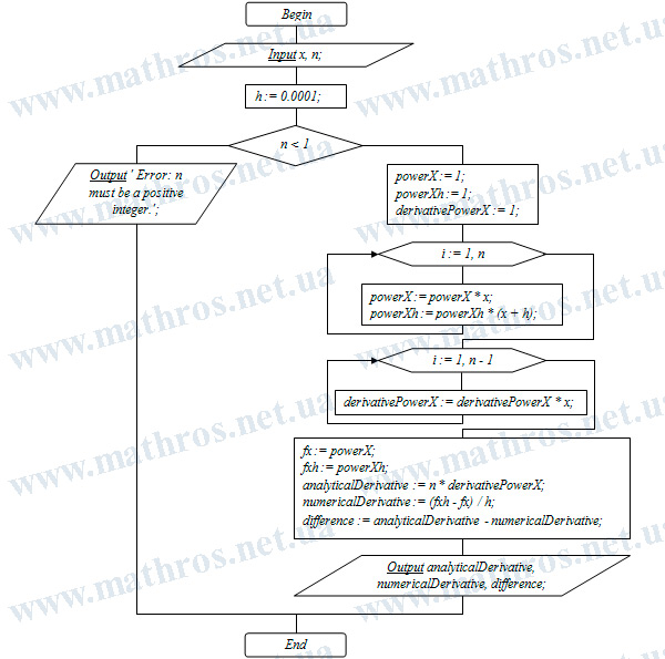
Power Rule: An Algorithm for Programmatic Verification
If you enjoy programming, try looking at the power rule not only as a mathematical formula, but also as a ready-made algorithm for calculations. Using a flowchart, you can implement a program in any convenient language: Pascal, Python, C++, JavaScript, or another one.
The idea is simple but interesting: the user enters \( n \) and \( x \), and the program calculates the derivative at this point in two ways — analytically using the power rule and numerically using a small increment. Then the results are compared. Isn’t this a great way to see how mathematical theory turns into working code?