The Newton–Leibniz formula establishes a connection between a definite integral and an antiderivative of a function. Thanks to this relationship, calculating an integral comes down to finding an antiderivative and evaluating it at the limits of integration. How exactly does this formula work, and what should you pay attention to when using it? Let’s go through it step by step.
Newton–Leibniz Formula: Calculating a Definite Integral
Let the function \( f(x) \) be continuous on the interval \( [a,b] \), and let \( F(x) \) be one of its antiderivatives. That is,
\[
F'(x)=f(x).
\]
Then the definite integral can be calculated using the formula
\[
\int_a^b f(x)\,dx=F(b)-F(a).
\]
This is the Newton–Leibniz formula. It shows that to find the value of a definite integral, you only need to find an antiderivative \( F(x) \), calculate \( F(b) \), and subtract \( F(a) \).
The formula is also often written in a shorter form:
\[
\int_a^b f(x)\,dx=\left.F(x)\right|_a^b,
\]
where the notation
\[
\left.F(x)\right|_a^b
\]
means
\[
F(b)-F(a).
\]
So, the order of the limits matters. First, calculate the value of the antiderivative at the upper limit, and then subtract its value at the lower limit.
A natural question comes up: which antiderivative should you use? After all, the same function has infinitely many antiderivatives that differ by a constant:
\[
F_1(x)=F(x)+C.
\]
However, this constant does not affect the value of the definite integral because
\[
F_1(b)-F_1(a)=F(b)+C-\bigl(F(a)+C\bigr)=F(b)-F(a).
\]
That is why there is no need to write the constant \( C \) when calculating a definite integral.
So, once you have found an antiderivative, it is enough to calculate \( F(b) \) and \( F(a) \), and then find their difference. It is important to remember that you evaluate the antiderivative \( F(x) \) at the limits of integration, not the original function \( f(x) \).
In addition, the Newton–Leibniz formula directly shows that reversing the order of the limits changes the sign of the integral:
\[
\int_b^a f(x)\,dx=F(a)-F(b)
=-\bigl(F(b)-F(a)\bigr),
\]
so
\[
\int_b^a f(x)\,dx=-\int_a^b f(x)\,dx.
\]
If the limits of integration are the same, then
\[
\int_a^a f(x)\,dx=F(a)-F(a)=0.
\]
Thus, the Newton–Leibniz formula makes it possible to reduce the calculation of a definite integral to evaluating an antiderivative. The key is to find the antiderivative correctly, keep the limits in the right order, and evaluate it carefully at each limit.
Newton–Leibniz Formula: Practical Examples of Definite Integrals
After learning the Newton–Leibniz formula, it is useful to see how it works in actual calculations. In each case, we will first find an antiderivative and then evaluate it at the limits of integration.
Example 1. Calculate the definite integral
\[
\int_0^2 (3\cdot x^2+2\cdot x)\,dx.
\]
First, find the indefinite integral of the integrand:
\[
\int (3\cdot x^2+2\cdot x)\,dx=x^3+x^2+C.
\]
Therefore, we can choose the antiderivative
\[
F(x)=x^3+x^2.
\]
Now apply the Newton–Leibniz formula:
\[
\int_0^2 (3\cdot x^2+2\cdot x)\,dx
=
\left.(x^3+x^2)\right|_0^2.
\]
Substitute the upper limit:
\[
F(2)=2^3+2^2=8+4=12.
\]
Next, substitute the lower limit:
\[
F(0)=0^3+0^2=0.
\]
Find the difference:
\[
F(2)-F(0)=12-0=12.
\]
Therefore,
\[
\int_0^2 (3\cdot x^2+2\cdot x)\,dx=12.
\]
Example 2. Calculate the definite integral
\[
\int_0^{\frac{\pi}{2}}\cos(x)\,dx.
\]
An antiderivative of \( \cos(x) \) is
\[
F(x)=\sin(x),
\]
because
\[
(\sin(x))’=\cos(x).
\]
Using the Newton–Leibniz formula, we get
\[
\int_0^{\frac{\pi}{2}}\cos(x)\,dx
=
\left.\sin(x)\right|_0^{\frac{\pi}{2}}.
\]
First, calculate the value of the antiderivative at the upper limit:
\[
F\left(\frac{\pi}{2}\right)
=
\sin\left(\frac{\pi}{2}\right)
=
1.
\]
Then find the value of the antiderivative at the lower limit:
\[
F(0)=\sin(0)=0.
\]
Therefore,
\[
F\left(\frac{\pi}{2}\right)-F(0)=1-0=1.
\]
So,
\[
\int_0^{\frac{\pi}{2}}\cos(x)\,dx=1.
\]
Example 3. Calculate the definite integral
\[
\int_1^e \frac{1}{x}\,dx.
\]
An antiderivative of the function
\[
\frac{1}{x}
\]
is
\[
F(x)=\ln(x),
\]
because
\[
(\ln(x))’=\frac{1}{x}.
\]
Therefore, using the Newton–Leibniz formula,
\[
\int_1^e \frac{1}{x}\,dx
=
\left.\ln(x)\right|_1^e.
\]
First, calculate the value of the antiderivative at the upper limit:
\[
F(e)=\ln(e)=1.
\]
Now substitute the lower limit:
\[
F(1)=\ln(1)=0.
\]
Find the difference:
\[
F(e)-F(1)=1-0=1.
\]
Therefore,
\[
\int_1^e \frac{1}{x}\,dx=1.
\]
Example 4. Calculate the definite integral
\[
\int_1^4 \frac{1}{\sqrt{x}}\,dx.
\]
First, rewrite the integrand in power form:
\[
\frac{1}{\sqrt{x}}=x^{-\frac{1}{2}}.
\]
Then
\[
\int x^{-\frac{1}{2}}\,dx
=
\frac{x^{\frac{1}{2}}}{\frac{1}{2}}+C
=
2\cdot\sqrt{x}+C.
\]
Therefore, we can choose the antiderivative
\[
F(x)=2\cdot\sqrt{x}.
\]
Using the Newton–Leibniz formula,
\[
\int_1^4 \frac{1}{\sqrt{x}}\,dx
=
\left.2\cdot\sqrt{x}\right|_1^4.
\]
Calculate the value of the antiderivative at the upper limit:
\[
F(4)=2\cdot\sqrt{4}=2\cdot2=4.
\]
Now find the value of the antiderivative at the lower limit:
\[
F(1)=2\cdot\sqrt{1}=2.
\]
Therefore,
\[
F(4)-F(1)=4-2=2.
\]
So,
\[
\int_1^4 \frac{1}{\sqrt{x}}\,dx=2.
\]
Example 5. Calculate the definite integral
\[
\int_2^{-1}(2\cdot x-3)\,dx.
\]
Notice that the upper limit is smaller than the lower limit. However, the Newton–Leibniz formula can still be applied directly without reversing the limits.
Find the indefinite integral:
\[
\int (2\cdot x-3)\,dx=x^2-3\cdot x+C.
\]
Therefore, we can choose the antiderivative
\[
F(x)=x^2-3\cdot x.
\]
Apply the Newton–Leibniz formula:
\[
\int_2^{-1}(2\cdot x-3)\,dx
=
\left.(x^2-3\cdot x)\right|_2^{-1}.
\]
First, substitute the upper limit \( -1 \):
\[
F(-1)=(-1)^2-3\cdot(-1)=1+3=4.
\]
Next, substitute the lower limit \( 2 \):
\[
F(2)=2^2-3\cdot2=4-6=-2.
\]
Now find the difference:
\[
F(-1)-F(2)=4-(-2)=6.
\]
Therefore,
\[
\int_2^{-1}(2\cdot x-3)\,dx=6.
\]
Next Step in Integral Calculus: Topics to Explore
After learning the Newton–Leibniz formula, it is natural to move on to problems where the definite integral takes on a geometric meaning. The following topics will show how definite integrals are used to calculate areas, volumes, and lengths.
- Area of a Region Using an Integral: Formulas and Examples — This article will explain how to use a definite integral to find the area of regions bounded by graphs of functions and straight lines.
- Volume of a Solid of Revolution: Applying the Definite Integral — This article will explain how the definite integral can be used to calculate the volumes of solids formed by rotating plane regions.
- Arc Length of a Curve: Formula Using a Definite Integral — This article will cover how to calculate the arc length of the graph of a function and explain the role of the definite integral in such problems.
Newton–Leibniz Formula: From Mathematics to Programming
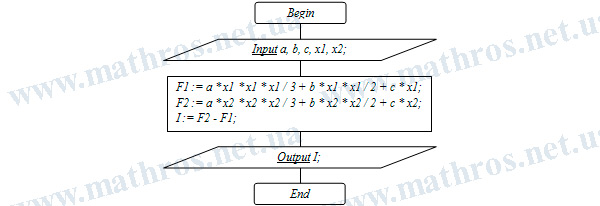
If you enjoy programming, try turning what you have learned about the Newton–Leibniz formula into your own code. The flowchart below shows an algorithm for calculating the definite integral of the function
\[
f(x)=a\cdot x^2+b\cdot x+c.
\]
The algorithm takes the coefficients of the function and the limits of integration, calculates the value of the antiderivative at each limit, and finds the difference between these two values. Implement this algorithm in your favorite programming language and test it with different input values.