The coordinate descent method is one of those numerical methods that are convenient to study gradually, step by step. Why is that so? Because it does not change all variables at the same time. Instead, the search for the minimum is performed one coordinate at a time. Thanks to this, a complex minimization problem for a function of several variables becomes much simpler.
In addition, this approach works well for learning purposes. It allows us to see how the algorithm is built, how a new approximation is formed, and when it makes sense to stop the calculations. Next, we will look step by step at the main idea of the method, the structure of one complete cycle, and the stopping conditions.
Coordinate Descent Method: Where It Is Used and What Its Main Idea Is
Suppose we are given a function of several variables
\[
f(\bar{x})=f(x_1,x_2,\dots,x_n),
\]
where \( \bar{x} \) is the vector of variables. We need to find the minimum point of this function or an approximation to a local minimum point. This is exactly the type of problem where the coordinate descent method is used.
The main idea is that at each stage, only one variable is changed, while all the other variables are considered fixed. As a result, a multidimensional minimization problem is broken down into a sequence of one-dimensional problems. And that is much easier both for analysis and for calculations.
We start with some initial approximation
\[
\bar{x}^{(0)}=\bigl(x_1^{(0)},x_2^{(0)},\dots,x_n^{(0)}\bigr).
\]
After that, the search for the minimum is performed along each coordinate one by one. First, we change \( x_1 \), then \( x_2 \), then \( x_3 \), and so on until \( x_n \).
When is this approach convenient? First of all, when minimization with respect to each separate coordinate can be performed relatively simply. In addition, it is important that the function is defined at the points through which the search process passes. That is why the coordinate descent method is often considered one of the basic approaches in numerical optimization.
At the same time, one important clarification should be made right away. In the general case, this method leads to an approximation of a local minimum, not necessarily a global one. Therefore, the obtained result may depend on the choice of the initial approximation.
Minimization by Coordinates: What One Complete Cycle Looks Like
After choosing the initial approximation, we can move on to the description of the computational process itself. Suppose we have the point
\[
\bar{x}^{(0)}=\bigl(x_1^{(0)},x_2^{(0)},\dots,x_n^{(0)}\bigr).
\]
At the first step, we fix all coordinates except \( x_1 \) and consider a function of one variable:
\[
\varphi_1(x_1)=f(x_1,x_2^{(0)},\dots,x_n^{(0)}).
\]
Next, we find the value of \( x_1 \) at which this function reaches its minimum. Let this value be \( x_1^{(1)} \). Then, after the first step, we obtain a new intermediate approximation: \( \bigl(x_1^{(1)},x_2^{(0)},\dots,x_n^{(0)}\bigr) \).
After that, we move on to the second coordinate. Now we fix the already updated value \( x_1^{(1)} \), as well as all other coordinates except \( x_2 \), and consider the function
\[
\varphi_2(x_2)=f(x_1^{(1)},x_2,\dots,x_n^{(0)}).
\]
After finding its minimum, we obtain a new intermediate approximation: \( \bigl(x_1^{(1)},x_2^{(1)},\dots,x_n^{(0)}\bigr) \).
In the same way, the process continues for all other coordinates up to \( x_n \). After all variables have been processed once, we obtain a new point
\[
\bar{x}^{(1)}=\bigl(x_1^{(1)},x_2^{(1)},\dots,x_n^{(1)}\bigr).
\]
This transition from \( \bar{x}^{(0)} \) to \( \bar{x}^{(1)} \) is called one complete cycle of the method.
Here, it is important not to confuse two concepts.
- A step of the method is minimization with respect to one coordinate.
- A complete cycle is the sequential execution of such steps for all coordinates.
After each update of a separate coordinate, the value of the function usually does not increase. Therefore, after completing a complete cycle, we also have
\[
f\bigl(\bar{x}^{(1)}\bigr)\leq f\bigl(\bar{x}^{(0)}\bigr).
\]
If we then perform one more cycle, we obtain the point \( \bar{x}^{(2)} \), and in this case we have
\[
f\bigl(\bar{x}^{(2)}\bigr)\leq f\bigl(\bar{x}^{(1)}\bigr)\leq f\bigl(\bar{x}^{(0)}\bigr).
\]
So, we get a sequence of approximations
\[
\bar{x}^{(0)},\bar{x}^{(1)},\bar{x}^{(2)},\dots
\]
for which the values of the objective function form a monotonically non-increasing sequence.
Thus, after describing one complete cycle, the main logic of the algorithm becomes clear: each new cycle improves the previous approximation, while the function value gradually decreases or at least remains at the same level.
Coordinate Descent Method: When It Makes Sense to Stop the Calculations
After the structure of one complete cycle has become clear, a natural question appears: when exactly should we stop the computational process? After all, the cycles can be repeated many times. However, in practice, the algorithm is stopped when further changes become sufficiently small.
Here, it is important to emphasize one point: the stopping condition is most often checked after a complete cycle, not after each separate step. Why is that so? Because after one step, only one coordinate changes, while after a complete cycle, the whole point is updated:
\[
\bar{x}^{(k)}=(x_1^{(k)},x_2^{(k)},\dots,x_n^{(k)}).
\]
That is why it is logical to compare the approximations \( \bar{x}^{(k)} \) and \( \bar{x}^{(k+1)} \), obtained after two consecutive complete cycles.
One of the most commonly used stopping criteria is related to the change in the point itself:
\[
\|\bar{x}^{(k+1)}-\bar{x}^{(k)}\|<\varepsilon,
\]
where \( \varepsilon>0 \) is the given accuracy. Here, the norm shows how much the new approximation differs from the previous one as a whole across all coordinates. If this difference is already very small, the process can be stopped.
Another common criterion is related to the change in the function value:
\[
\bigl|f(\bar{x}^{(k+1)})-f(\bar{x}^{(k)})\bigr|<\varepsilon.
\]
In this case, we check whether the improvement in the function value has become sufficiently small. If so, further cycles no longer give a significant result.
In addition, sometimes a limit is set on the maximum number of complete cycles:
\[
k\geq k_{\max}.
\]
This criterion is needed so that the algorithm does not run for too long if convergence is slow.
In practice, several stopping conditions are often used at the same time. This is convenient because it allows us to control the change in the point, the change in the function value, and the overall duration of the calculations.
So, the coordinate descent method is a sequential process of minimization along separate coordinates. It is repeated until the chosen stopping condition is satisfied.
Practical Part: How the Method Works in an Example
Now let us move on to a concrete example of applying the coordinate descent method. A practical problem is the best way to see how the coordinates change step by step, how a new approximation is formed, and when the calculations can be stopped.
Example 1. Find the minimum value of the function \( f(x_1,x_2)=x_1^2+x_1\cdot x_2+x_2^2-6\cdot x_1-4\cdot x_2 \) with accuracy \( \varepsilon=0.05 \), using the coordinate descent method
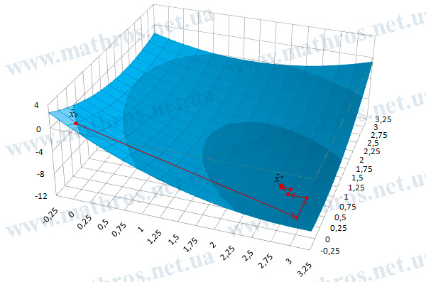
Let us consider the given function of two variables. It is a quadratic function, and therefore it is sufficiently smooth for applying the coordinate descent method. We take the initial approximation
\[
\bar{x}^{(0)}=(0,0).
\]
We will check the stopping condition after each complete cycle according to the rule
\[
\|\bar{x}^{(k+1)}-\bar{x}^{(k)}\|<0.05.
\]
Here, it is important to note right away that in this example, minimization with respect to each coordinate is performed not by using a separate numerical one-dimensional method, such as the dichotomy method, the Fibonacci method, or the golden section method. Instead, we find the minimum of the corresponding one-dimensional quadratic function exactly, using the derivative. This approach makes it easier to see the main logic of the coordinate descent method without adding extra complexity through intermediate numerical procedures.
We begin the first complete cycle. First, we fix \( x_2=0 \) and minimize the function with respect to \( x_1 \). Then we have
\[
\varphi_1(x_1)=f(x_1,0)=x_1^2-6\cdot x_1.
\]
Let us calculate the derivative:
\[
\varphi_1′(x_1)=2\cdot x_1-6.
\]
Next, we set it equal to zero:
\[
2\cdot x_1-6=0.
\]
From this, we get
\[
x_1^{(1)}=3.
\]
So, after the first step, we have the intermediate approximation \( (3,0) \).
Now we fix \( x_1=3 \) and minimize the function with respect to \( x_2 \):
\[
\varphi_2(x_2)=f(3,x_2)=3^2+3\cdot x_2+x_2^2-6\cdot 3-4\cdot x_2.
\]
After simplification, we get
\[
\varphi_2(x_2)=x_2^2-x_2-9.
\]
Then
\[
\varphi_2′(x_2)=2\cdot x_2-1.
\]
We set it equal to zero:
\[
2\cdot x_2-1=0.
\]
Therefore,
\[
x_2^{(1)}=0.5.
\]
After completing the first complete cycle, we obtain the point
\[
\bar{x}^{(1)}=(3,0.5).
\]
Let us calculate the value of the function at this point:
\[
f\bigl(\bar{x}^{(1)}\bigr)=f(3,0.500)=-9.250.
\]
Now we check whether the accuracy condition is satisfied:
\[
\|\bar{x}^{(1)}-\bar{x}^{(0)}\|
=\sqrt{(3-0)^2+(0.5-0)^2}
=\sqrt{9.25}\approx 3.041.
\]
Since
\[
3.041>0.05,
\]
we continue the calculations.
Continuation of the Iterative Process
We move on to the second complete cycle. We fix \( x_2=0.5 \) and consider the function
\[
\varphi_1(x_1)=f(x_1,0.5)=x_1^2+0.5\cdot x_1+0.25-6\cdot x_1-2.
\]
After simplification, we have
\[
\varphi_1(x_1)=x_1^2-5.5\cdot x_1-1.75.
\]
Then
\[
\varphi_1′(x_1)=2\cdot x_1-5.5.
\]
We set it equal to zero:
\[
2\cdot x_1-5.5=0.
\]
Hence,
\[
x_1=2.75.
\]
After that, we have the intermediate approximation \( (2.75,0.5) \).
Now we fix \( x_1=2.75 \) and minimize with respect to \( x_2 \):
\[
\varphi_2(x_2)=f(2.75,x_2)=2.75^2+2.75\cdot x_2+x_2^2-6\cdot 2.75-4\cdot x_2.
\]
After simplification, we obtain
\[
\varphi_2(x_2)=x_2^2-1.25\cdot x_2-8.938.
\]
Let us find the derivative:
\[
\varphi_2′(x_2)=2\cdot x_2-1.25.
\]
We set it equal to zero:
\[
2\cdot x_2-1.25=0.
\]
Therefore,
\[
x_2=0.625.
\]
After the second complete cycle, we get the point
\[
\bar{x}^{(2)}=(2.75,0.625).
\]
Let us calculate the function value:
\[
f\bigl(\bar{x}^{(2)}\bigr)=f(2.75,0.625)\approx -9.328.
\]
Again, we check whether the accuracy condition is satisfied:
\[
\|\bar{x}^{(2)}-\bar{x}^{(1)}\|
=\sqrt{(2.75-3)^2+(0.625-0.5)^2}
\approx 0.28.
\]
Since
\[
0.28>0.05,
\]
we move on to the next cycle.
Let us consider the third complete cycle. First, we fix \( x_2=0.625 \). Then
\[
\varphi_1(x_1)=f(x_1,0.625)=x_1^2+0.625\cdot x_1+0.391-6\cdot x_1-2.5.
\]
After simplification, we have
\[
\varphi_1(x_1)=x_1^2-5.375\cdot x_1-2.109.
\]
Its derivative is
\[
\varphi_1′(x_1)=2\cdot x_1-5.375.
\]
We set it equal to zero:
\[
2\cdot x_1-5.375=0.
\]
Therefore,
\[
x_1=2.688.
\]
Next, we fix \( x_1=2.688 \) and minimize the function with respect to \( x_2 \):
\[
\varphi_2(x_2)=f(2.688,x_2)=2.688^2+2.688\cdot x_2+x_2^2-6\cdot 2.688-4\cdot x_2.
\]
After simplification, we obtain
\[
\varphi_2(x_2)=x_2^2-1.312\cdot x_2-8.903.
\]
Then
\[
\varphi_2′(x_2)=2\cdot x_2-1.312.
\]
We set it equal to zero:
\[
2\cdot x_2-1.312=0.
\]
Hence,
\[
x_2=0.656.
\]
So, after the third complete cycle, we have the point
\[
\bar{x}^{(3)}=(2.688,0.656).
\]
Let us calculate the function value:
\[
f\bigl(\bar{x}^{(3)}\bigr)=f(2.688,0.656)\approx -9.333.
\]
We check whether the accuracy condition is satisfied:
\[
\|\bar{x}^{(3)}-\bar{x}^{(2)}\|
=\sqrt{(2.688-2.75)^2+(0.656-0.625)^2}
\approx 0.069.
\]
Since
\[
0.069>0.05,
\]
we perform one more cycle.
In the fourth complete cycle, we first fix \( x_2=0.656 \). Then we consider the function
\[
\varphi_1(x_1)=f(x_1,0.656)=x_1^2+0.656\cdot x_1+0.43-6\cdot x_1-2.624.
\]
After simplification, we have
\[
\varphi_1(x_1)=x_1^2-5.344\cdot x_1-2.194.
\]
Its derivative is
\[
\varphi_1′(x_1)=2\cdot x_1-5.344.
\]
We set it equal to zero:
\[
2\cdot x_1-5.344=0.
\]
Hence,
\[
x_1=2.672.
\]
After that, we fix \( x_1=2.672 \) and consider the function with respect to \( x_2 \):
\[
\varphi_2(x_2)=f(2.672,x_2)=2.672^2+2.672\cdot x_2+x_2^2-6\cdot 2.672-4\cdot x_2.
\]
After simplification, we get
\[
\varphi_2(x_2)=x_2^2-1.328\cdot x_2-8.892.
\]
Then
\[
\varphi_2′(x_2)=2\cdot x_2-1.328.
\]
We set it equal to zero:
\[
2\cdot x_2-1.328=0.
\]
Therefore,
\[
x_2=0.664.
\]
After the fourth complete cycle, we obtain
\[
\bar{x}^{(4)}=(2.672,0.664).
\]
Now we check the stopping condition again:
\[
\|\bar{x}^{(4)}-\bar{x}^{(3)}\|
=\sqrt{(2.672-2.688)^2+(0.664-0.656)^2}
\approx 0.018.
\]
Since
\[
0.018<0.05,
\]
the iterative process can be stopped.
Let us calculate the value of the function at the last point found:
\[
f\bigl(\bar{x}^{(4)}\bigr)=f(2.672,0.664)\approx -9.333.
\]
Therefore, the approximate minimum point is
\[
\bar{x}^{*}\approx (2.672,0.664),
\]
and the approximate minimum value of the function is
\[
f_{\min}\approx -9.333.
\]
Comparison with the Exact Answer
Let us check how this result agrees with the exact answer. To do this, we solve the system of stationarity conditions:
\[
\frac{\partial f}{\partial x_1}=2\cdot x_1+x_2-6=0,
\qquad
\frac{\partial f}{\partial x_2}=x_1+2\cdot x_2-4=0.
\]
From this, we get
\[
x_1=\frac{8}{3}\approx 2.667,
\qquad
x_2=\frac{2}{3}\approx 0.667.
\]
The corresponding exact minimum value is
\[
f\left(\frac{8}{3},\frac{2}{3}\right)
=-\frac{28}{3}\approx -9.333.
\]
In addition, in this example, we can show that the minimum found is not only local but also global. Indeed, the matrix of second derivatives has the form
\[
H=
\begin{pmatrix}
2 & 1\\
1 & 2
\end{pmatrix}.
\]
Its leading principal minors satisfy the conditions
\[
2>0,
\qquad
\det(H)=4-1=3>0.
\]
Therefore, the matrix \( H \) is positive definite, and the function is strictly convex. That is why the point
\[
\left(\frac{8}{3},\frac{2}{3}\right)
\]
is the unique global minimum point.
Thus, this example clearly shows the full path of applying the coordinate descent method: from choosing the initial approximation and constructing one-dimensional functions to checking the accuracy, calculating the function value after each complete cycle, and finding the minimum value. At the same time, it clearly demonstrates that in this case, minimization with respect to each coordinate was performed analytically using the derivative, without using separate numerical methods for one-dimensional minimization.
What to Consider Next: Useful Topics for Further Study
We have already looked at the coordinate descent method step by step: from the main idea to a practical example. However, the study of minimization methods does not end here. What else is worth reading next to better understand the differences between these approaches and their capabilities?
- Gradient Descent Method: How to Move in the Direction of the Fastest Decrease — In this article, we will discuss how to find the minimum of a function of several variables using the direction of the steepest decrease.
- Newton’s Method: How to Use Second Derivatives to Find a Minimum — In this article, we will discuss how Newton’s method helps find the minimum point of a function of several variables and why it often converges faster.
- Newton’s Method with a Parameter: How to Control the Search Step — In this article, we will discuss how a parameter in Newton’s method affects the calculation process and makes the search more stable.
Programming Practice: Try to Implement the Algorithm Yourself
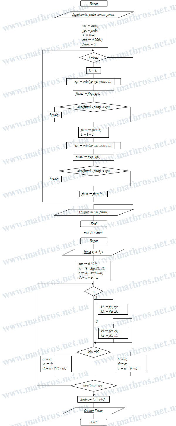
If you are interested not only in reading about the method but also in seeing how it works in a program, pay attention to the flowchart below. It can become a convenient basis for creating a small program in your favorite programming language that finds the minimum value of a function of several variables using the coordinate descent method.
Such an attempt helps you understand the algorithm better, see the connection between mathematical notation and code, and at the same time test how the method works on different functions. This is no longer just theory, but a fully practical step toward your own implementation.