Linear interpolation is one of the simplest methods for approximating function values from known tabulated data. It is used when we need to find a function value between two adjacent nodes without constructing a high-degree interpolation polynomial. First, we will look at how a linear interpolation polynomial is constructed, and then we will use it to solve practical examples.
Linear Interpolation: The Idea of Approximation Between Nodes
Suppose a function is given by a table of values at the nodes
\[
(x_0,y_0),\quad(x_1,y_1),\quad\dots,\quad(x_n,y_n),
\]
where the argument values are ordered as follows:
\[
x_0<x_1<\dots<x_n.
\]
This ordering makes it possible to clearly identify adjacent nodes and the corresponding intervals between them. The nodes do not have to be equally spaced: for linear interpolation, it is enough to know the coordinates of two adjacent points with different \( x \)-values.
If there are many nodes, constructing a single interpolation polynomial for the entire interval can be inconvenient because its degree increases with the number of given points. A simpler approach is to consider each pair of adjacent nodes separately.
The points \( (x_i,y_i) \) and \( (x_{i+1},y_{i+1}) \) are connected by a straight line segment. On the interval between these nodes, the given function is approximated by this line.
If this construction is carried out for all adjacent pairs of nodes, we obtain a piecewise linear curve whose vertices coincide with the given points. This method of approximation is called piecewise linear interpolation.
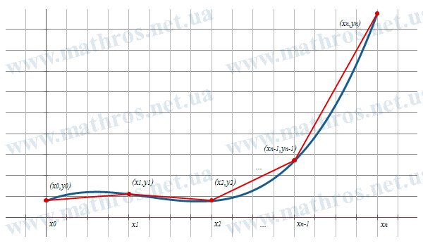
On each individual interval
\[
x_i\leq x\leq x_{i+1}
\]
the approximation is defined by a first-degree polynomial
\[
F(x)=a\cdot x+b.
\]
For different intervals, the coefficients \( a \) and \( b \) may have different values because each straight line is constructed from its own pair of adjacent nodes. Thus, instead of using a single high-degree polynomial, we use a set of linear polynomials, each of which describes the function on the corresponding interval.
Linear Interpolation Polynomial: Determining the Coefficients
To construct a linear polynomial on the interval between the nodes \( (x_i,y_i) \) and \( (x_{i+1},y_{i+1}) \), we need to determine its coefficients \( a \) and \( b \):
\[
F(x)=a\cdot x+b.
\]
Since the straight line must pass through both given nodes, we have the conditions
\[
y_i=a\cdot x_i+b,\qquad y_{i+1}=a\cdot x_{i+1}+b.
\]
Therefore, the coefficients are determined from the following system of two linear equations:
\[
\begin{cases}
y_i=a\cdot x_i+b,\\
y_{i+1}=a\cdot x_{i+1}+b.
\end{cases}
\]
Subtracting the first equation from the second, we obtain
\[
y_{i+1}-y_i=a\cdot(x_{i+1}-x_i).
\]
Hence,
\[
a=\frac{y_{i+1}-y_i}{x_{i+1}-x_i}.
\]
The coefficient \( a \) determines the slope of the line and shows how the value of the linear polynomial changes when the argument increases by one unit. Since ( x_{i+1}\neq x_i ), the denominator in this formula is not equal to zero.
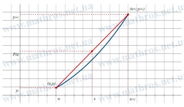
After finding \( a \), we determine the coefficient \( b \) from the first equation:
\[
b=y_i-a\cdot x_i.
\]
Substituting the obtained coefficients into the equation of the line and simplifying, we get the linear interpolation polynomial:
\[
F(x)=y_i+\frac{y_{i+1}-y_i}{x_{i+1}-x_i}\cdot(x-x_i),\qquad x_i\leq x\leq x_{i+1}.
\]
This formula allows us to directly determine an approximate function value from the coordinates of two adjacent nodes. If we substitute \( x=x_i \), we obtain
\[
F(x_i)=y_i,
\]
and for \( x=x_{i+1} \),
\[
F(x_{i+1})=y_{i+1}.
\]
Thus, at the nodes themselves, the interpolation polynomial reproduces the given function values exactly. The values calculated between adjacent nodes are approximate.
Linear Interpolation: Step-by-Step Examples
Now let us move on to the practical use of linear interpolation for tabulated data with unequally spaced nodes. In each case, we will identify the adjacent nodes between which the given argument value lies and use them to calculate the approximate function value.
Example 1. Using the tabulated function values below, find the approximate value of \( f(2.1) \)
| \( i \) | \( x_i \) | \( y_i \) |
|---|---|---|
| \( 0 \) | \( 0 \) | \( 2 \) |
| \( 1 \) | \( 1.5 \) | \( 5 \) |
| \( 2 \) | \( 3.2 \) | \( 9 \) |
First, determine between which adjacent nodes the given argument value lies:
\[
1.5<2.1<3.2.
\]
Therefore, for interpolation we use the points
\[
(x_i,y_i)=(1.5,5)
\]
and
\[
(x_{i+1},y_{i+1})=(3.2,9).
\]
Write the formula for the linear interpolation polynomial:
\[
F(x)=y_i+\frac{y_{i+1}-y_i}{x_{i+1}-x_i}\cdot(x-x_i).
\]
Substitute the coordinates of the selected nodes:
\[
F(x)=5+\frac{9-5}{3.2-1.5}\cdot(x-1.5).
\]
For \( x=2.1 \), we have
\[
F(2.1)=5+\frac{9-5}{3.2-1.5}\cdot(2.1-1.5).
\]
Calculate the differences:
\[
9-5=4,\qquad 3.2-1.5=1.7,\qquad 2.1-1.5=0.6.
\]
Then
\[
F(2.1)=5+\frac{4}{1.7}\cdot0.6\approx5+1.412=6.412.
\]
Therefore,
\[
f(2.1)\approx6.412.
\]
Example 2. Using the tabulated function values below, find the approximate value of \( f(5.2) \)
| \( i \) | \( x_i \) | \( y_i \) |
|---|---|---|
| \( 0 \) | \( 1 \) | \( 3 \) |
| \( 1 \) | \( 2.4 \) | \( 6.5 \) |
| \( 2 \) | \( 4 \) | \( 9 \) |
| \( 3 \) | \( 7 \) | \( 15 \) |
Determine between which adjacent nodes the value \( x=5.2 \) lies:
\[
4<5.2<7.
\]
Therefore, for interpolation we use the points
\[
(x_i,y_i)=(4,9)
\]
and
\[
(x_{i+1},y_{i+1})=(7,15).
\]
Substitute the coordinates of the selected nodes into the linear interpolation formula:
\[
F(x)=9+\frac{15-9}{7-4}\cdot(x-4).
\]
For \( x=5.2 \), we obtain
\[
F(5.2)=9+\frac{15-9}{7-4}\cdot(5.2-4).
\]
Calculate the differences:
\[
15-9=6,\qquad 7-4=3,\qquad 5.2-4=1.2.
\]
Then
\[
F(5.2)=9+\frac{6}{3}\cdot1.2=9+2.4=11.4.
\]
Therefore,
\[
f(5.2)\approx11.4.
\]
Example 3. Using the tabulated function values below, find the approximate value of \( f(0.7) \)
| \( i \) | \( x_i \) | \( y_i \) |
|---|---|---|
| \( 0 \) | \( -2 \) | \( 4 \) |
| \( 1 \) | \( -0.5 \) | \( 1.5 \) |
| \( 2 \) | \( 1.8 \) | \( 5.2 \) |
| \( 3 \) | \( 3 \) | \( 8 \) |
| \( 4 \) | \( 6.5 \) | \( 20 \) |
Determine between which adjacent nodes the value \( x=0.7 \) lies:
\[
-0.5<0.7<1.8.
\]
Therefore, we use the points
\[
(x_i,y_i)=(-0.5,1.5)
\]
and
\[
(x_{i+1},y_{i+1})=(1.8,5.2).
\]
Substitute the coordinates of the selected nodes into the linear interpolation formula:
\[
F(x)=1.5+\frac{5.2-1.5}{1.8-(-0.5)}\cdot(x-(-0.5)).
\]
For \( x=0.7 \), we have
\[
F(0.7)=1.5+\frac{5.2-1.5}{1.8-(-0.5)}\cdot(0.7-(-0.5)).
\]
Calculate the differences:
\[
5.2-1.5=3.7,\qquad 1.8-(-0.5)=2.3,\qquad 0.7-(-0.5)=1.2.
\]
Then
\[
F(0.7)=1.5+\frac{3.7}{2.3}\cdot1.2.
\]
Carrying out the calculation, we get
\[
F(0.7)\approx1.5+1.93=3.43.
\]
Therefore,
\[
f(0.7)\approx3.43.
\]
Interpolation Methods: What to Explore Next
Linear interpolation clearly demonstrates the basic idea of approximation between adjacent nodes. Next, you can explore methods that allow you to build more advanced approximations for functions given by tabulated data.
- Quadratic Interpolation: Approximation Using Three Nodes — In this article, we will look at how to construct a quadratic polynomial from three adjacent nodes and use it to find an intermediate function value.
- Cubic Spline Interpolation: Smooth Approximation Between Nodes — We will explore how cubic splines create a consistent approximation over separate intervals and help calculate function values.
- Trigonometric Interpolation: Approximation of Periodic Functions — We will learn how to construct a trigonometric polynomial from tabulated values to approximate periodic functions.
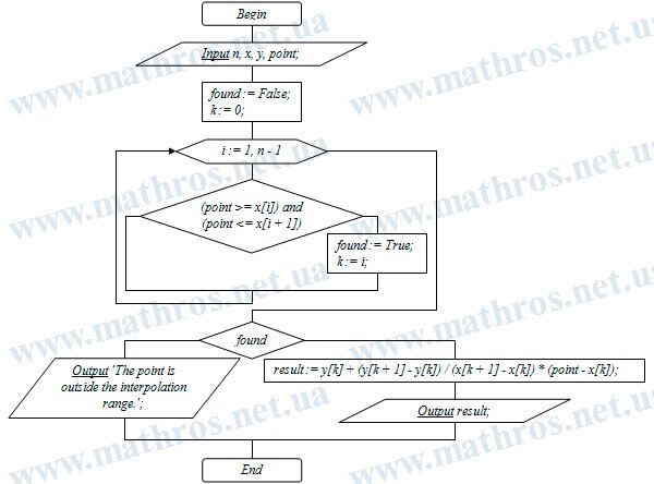
Linear Interpolation: From Flowchart to Program Code
If you enjoy programming, try turning the linear interpolation algorithm into your own program. Use the flowchart below as a guide: implement data input, find the interval containing the given argument value, and calculate the approximate function value. You can choose any programming language you prefer – Pascal, Python, JavaScript, C++, or another language. This is a good way to check how well you understand the algorithm and to see how the mathematical method works when implemented in code.