Eigenvalues of a matrix can be found in different ways. One of these ways is the Krylov method. It is useful when the characteristic polynomial is built using a special sequence of vectors.
At first glance, the method may seem complicated. However, its main idea is quite clear. First, we construct several vectors using the matrix \( A \). Then, based on these vectors, we form a system of linear equations. From this system, we find the coefficients of the characteristic polynomial. After that, we obtain the eigenvalues as the roots of the characteristic equation.
Eigenvalues of a Matrix: What Exactly Does the Krylov Method Find?
The Krylov method is used for a square matrix \( A \) of order \( n \). Its main goal is to find the characteristic polynomial of this matrix. Why exactly this polynomial? Because the roots of the characteristic polynomial are the eigenvalues of the matrix.
Let the characteristic polynomial of the matrix \( A \) have the form
\[
D(\lambda)=\det(\lambda\cdot I-A).
\]
Here, \( I \) is the identity matrix of the same order as the matrix \( A \).
After expanding the determinant, we obtain a polynomial of degree \( n \):
\[
D(\lambda)
=
\lambda^{n}
+
p_1\cdot\lambda^{n-1}
+
p_2\cdot\lambda^{n-2}
+
p_3\cdot\lambda^{n-3}
+
\dots
+
p_n.
\]
The numbers
\[
p_1,p_2,p_3,\dots,p_n
\]
are the coefficients of the characteristic polynomial. These are exactly the values that must first be found using the Krylov method.
So, the method does not begin with directly finding the eigenvalues. First, it helps determine the coefficients of the polynomial. After that, we write the characteristic equation
\[
D(\lambda)=0.
\]
Its roots
\[
\lambda_1,\lambda_2,\dots,\lambda_n
\]
are the eigenvalues of the matrix \( A \).
Thus, the logic of the method looks like this:
\[
A
\quad \longrightarrow \quad
D(\lambda)
\quad \longrightarrow \quad
D(\lambda)=0
\quad \longrightarrow \quad
\lambda_1,\lambda_2,\dots,\lambda_n.
\]
In other words, at first we work not with the eigenvalues themselves, but with the characteristic polynomial. This is important to understand from the very beginning, because this approach is the basis of the Krylov method.
Characteristic Polynomial: Why the Krylov Method Works
Now we need to explain where the main equality of the method comes from. For this, we use the Cayley–Hamilton theorem. It states that every square matrix satisfies its own characteristic equation.
Since the characteristic polynomial has the form
\[
D(\lambda)
=
\lambda^{n}
+
p_1\cdot\lambda^{n-1}
+
p_2\cdot\lambda^{n-2}
+
p_3\cdot\lambda^{n-3}
+
\dots
+
p_n,
\]
then for the matrix \( A \) itself, we can write:
\[
D(A)=0.
\]
Let us write this equality in more detail:
\[
A^{n}
+
p_1\cdot A^{n-1}
+
p_2\cdot A^{n-2}
+
p_3\cdot A^{n-3}
+
\dots
+
p_n\cdot I
=
0.
\]
This is a matrix equality. It shows that the powers of the matrix \( A \) are connected with one another through the coefficients of the characteristic polynomial.
In other words, the numbers
\[
p_1,p_2,p_3,\dots,p_n
\]
are the coefficients of this connection. These are exactly the coefficients we are looking for.
However, working directly with a matrix equation is not always convenient. Why? Because it contains powers of a matrix, and this can make the calculations more difficult, especially for matrices of higher order.
That is why the Krylov method takes the next step: it moves from a matrix equality to a vector equality. To do this, we introduce an initial vector and build a sequence of vectors connected with the matrix \( A \).
Krylov Vectors: Moving to a System of Equations
To move from a matrix equality to a vector equality, we choose any nonzero vector
\[
y^{(0)}
=
\begin{pmatrix}
y_1^{(0)}\\
y_2^{(0)}\\
y_3^{(0)}\\
\vdots\\
y_n^{(0)}
\end{pmatrix}.
\]
Its dimension must match the order of the matrix \( A \). In other words, if the matrix has order \( n \), then the vector \( y^{(0)} \) must also have \( n \) coordinates.
Why do we need this initial vector? It starts the construction of the whole sequence of vectors. Then each next vector is obtained by multiplying the matrix \( A \) by the previous vector.
First, we have
\[
y^{(1)}=A\cdot y^{(0)}.
\]
Then
\[
y^{(2)}=A\cdot y^{(1)}.
\]
Next,
\[
y^{(3)}=A\cdot y^{(2)}.
\]
In general, this process is written as
\[
y^{(i)}=A\cdot y^{(i-1)},
\qquad
i=1,2,3,\dots,n.
\]
Since each next multiplication adds one more factor \( A \), we can also write
\[
y^{(i)}=A^{i}\cdot y^{(0)},
\qquad
i=1,2,3,\dots,n.
\]
As a result, we obtain the sequence
\[
y^{(0)},y^{(1)},y^{(2)},\dots,y^{(n)}.
\]
These vectors are called Krylov vectors. They are needed to transform the matrix equality from the Cayley–Hamilton theorem into a more convenient vector equality.
Now let us return to the equality
\[
A^{n}
+
p_1\cdot A^{n-1}
+
p_2\cdot A^{n-2}
+
p_3\cdot A^{n-3}
+
\dots
+
p_n\cdot I
=
0.
\]
Multiply it on the right by the initial vector \( y^{(0)} \). We get
\[
A^{n}\cdot y^{(0)}
+
p_1\cdot A^{n-1}\cdot y^{(0)}
+
p_2\cdot A^{n-2}\cdot y^{(0)}
+
p_3\cdot A^{n-3}\cdot y^{(0)}
+
\dots
+
p_n\cdot y^{(0)}
=
0.
\]
Now we use the notation
\[
A^{i}\cdot y^{(0)}=y^{(i)}.
\]
Then the previous equality takes a simpler form:
\[
y^{(n)}
+
p_1\cdot y^{(n-1)}
+
p_2\cdot y^{(n-2)}
+
p_3\cdot y^{(n-3)}
+
\dots
+
p_n\cdot y^{(0)}
=
0.
\]
Next, move \( y^{(n)} \) to the right side:
\[
p_1\cdot y^{(n-1)}
+
p_2\cdot y^{(n-2)}
+
p_3\cdot y^{(n-3)}
+
\dots
+
p_n\cdot y^{(0)}
=
-y^{(n)}.
\]
This is already a vector equality. It is the basis for forming a system of linear equations.
Since each vector has \( n \) coordinates, this equality can be written as a system of \( n \) equations. The unknowns in this system will be the coefficients
\[
p_1,p_2,p_3,\dots,p_n.
\]
In coordinate form, this system looks like this:
\[
p_1\cdot y_j^{(n-1)}
+
p_2\cdot y_j^{(n-2)}
+
p_3\cdot y_j^{(n-3)}
+
\dots
+
p_n\cdot y_j^{(0)}
=
-y_j^{(n)},
\qquad
j=1,2,3,\dots,n.
\]
Or, in matrix form:
\[
\begin{pmatrix}
y_1^{(n-1)} & y_1^{(n-2)} & y_1^{(n-3)} & \dots & y_1^{(0)} \\
y_2^{(n-1)} & y_2^{(n-2)} & y_2^{(n-3)} & \dots & y_2^{(0)} \\
y_3^{(n-1)} & y_3^{(n-2)} & y_3^{(n-3)} & \dots & y_3^{(0)} \\
\vdots & \vdots & \vdots & \ddots & \vdots \\
y_n^{(n-1)} & y_n^{(n-2)} & y_n^{(n-3)} & \dots & y_n^{(0)}
\end{pmatrix}
\cdot
\begin{pmatrix}
p_1\\
p_2\\
p_3\\
\vdots\\
p_n
\end{pmatrix}
=
–
\begin{pmatrix}
y_1^{(n)}\\
y_2^{(n)}\\
y_3^{(n)}\\
\vdots\\
y_n^{(n)}
\end{pmatrix}.
\]
If this system has a unique solution, then the numbers found,
\[
p_1,p_2,p_3,\dots,p_n
\]
are the coefficients of the characteristic polynomial of the matrix \( A \). If the system does not have a unique solution, we usually choose another initial vector \( y^{(0)} \) and repeat the construction of Krylov vectors.
So, the Krylov method reduces the problem of finding eigenvalues to the construction of the characteristic polynomial through a system of linear equations. First, a sequence of vectors is formed. Then, using the Cayley–Hamilton theorem, we obtain a vector equality. From this equality, we build a system for the coefficients of the polynomial. This completes the theoretical basis of the method.
Practical Part: How the Krylov Method Works in Examples
Now let us move from the theoretical explanation to specific calculations. Using matrices of different orders, we will show how the Krylov method is applied and how the characteristic polynomial is gradually obtained. This makes it easier to see how the method works in real computations.
Example 1. Find the eigenvalues of a matrix using the Krylov method
\[
A=
\begin{pmatrix}
2 & 1\\
1 & 2
\end{pmatrix}.
\]
Choose the initial nonzero vector
\[
y^{(0)}
=
\begin{pmatrix}
1\\
0
\end{pmatrix}.
\]
This choice is convenient for calculations because the vector is simple and has the required dimension. Since the matrix is of order two, we need to construct the vectors up to \( y^{(2)} \) inclusive.
First, find \( y^{(1)} \):
\[
y^{(1)}=A\cdot y^{(0)}
=
\begin{pmatrix}
2 & 1\\
1 & 2
\end{pmatrix}
\cdot
\begin{pmatrix}
1\\
0
\end{pmatrix}
=
\begin{pmatrix}
2\\
1
\end{pmatrix}.
\]
Now find \( y^{(2)} \):
\[
y^{(2)}=A\cdot y^{(1)}
=
\begin{pmatrix}
2 & 1\\
1 & 2
\end{pmatrix}
\cdot
\begin{pmatrix}
2\\
1
\end{pmatrix}
=
\begin{pmatrix}
5\\
4
\end{pmatrix}.
\]
For a second-order matrix, the characteristic polynomial has the form
\[
D(\lambda)=\lambda^2+p_1\cdot\lambda+p_2.
\]
According to the Krylov method, we use the equality
\[
p_1\cdot y^{(1)}+p_2\cdot y^{(0)}=-y^{(2)}.
\]
Substitute the vectors we have found:
\[
p_1\cdot
\begin{pmatrix}
2\\
1
\end{pmatrix}
+
p_2\cdot
\begin{pmatrix}
1\\
0
\end{pmatrix}
=
–
\begin{pmatrix}
5\\
4
\end{pmatrix}.
\]
We obtain the system of equations:
\[
\begin{cases}
2\cdot p_1+p_2=-5,\\
p_1=-4.
\end{cases}
\]
From the second equation, we have
\[
p_1=-4.
\]
Substitute this value into the first equation:
\[
2\cdot(-4)+p_2=-5.
\]
Hence,
\[
\begin{gathered}
-8+p_2=-5,
\\[4pt]
p_2=3.
\end{gathered}
\]
So,
\[
p_1=-4,\qquad p_2=3.
\]
Therefore, the characteristic polynomial has the form
\[
D(\lambda)=\lambda^2-4\cdot\lambda+3.
\]
Write the characteristic equation:
\[
\lambda^2-4\cdot\lambda+3=0.
\]
Factor the quadratic expression:
\[
\lambda^2-4\cdot\lambda+3
=
(\lambda-1)\cdot(\lambda-3).
\]
Then the characteristic equation can be written as
\[
(\lambda-1)\cdot(\lambda-3)=0.
\]
Therefore, for the given matrix
\[
A=
\begin{pmatrix}
2 & 1\\
1 & 2
\end{pmatrix}
\]
the eigenvalues are
\[
\lambda_1=1,\qquad \lambda_2=3.
\]
Example 2. Find the eigenvalues of a matrix using the Krylov method
\[
A=
\begin{pmatrix}
1 & 0 & 0\\
0 & 2 & 0\\
0 & 0 & 3
\end{pmatrix}.
\]
Choose the initial vector
\[
y^{(0)}
=
\begin{pmatrix}
1\\
1\\
1
\end{pmatrix}.
\]
Since the matrix is of order three, we need to construct the vectors \( y^{(1)} \), \( y^{(2)} \), and \( y^{(3)} \).
Start by calculating \( y^{(1)} \):
\[
y^{(1)}=A\cdot y^{(0)}
=
\begin{pmatrix}
1 & 0 & 0\\
0 & 2 & 0\\
0 & 0 & 3
\end{pmatrix}
\cdot
\begin{pmatrix}
1\\
1\\
1
\end{pmatrix}
=
\begin{pmatrix}
1\\
2\\
3
\end{pmatrix}.
\]
Next, find \( y^{(2)} \):
\[
y^{(2)}=A\cdot y^{(1)}
=
\begin{pmatrix}
1 & 0 & 0\\
0 & 2 & 0\\
0 & 0 & 3
\end{pmatrix}
\cdot
\begin{pmatrix}
1\\
2\\
3
\end{pmatrix}
=
\begin{pmatrix}
1\\
4\\
9
\end{pmatrix}.
\]
And one more vector:
\[
y^{(3)}=A\cdot y^{(2)}
=
\begin{pmatrix}
1 & 0 & 0\\
0 & 2 & 0\\
0 & 0 & 3
\end{pmatrix}
\cdot
\begin{pmatrix}
1\\
4\\
9
\end{pmatrix}
=
\begin{pmatrix}
1\\
8\\
27
\end{pmatrix}.
\]
For a third-order matrix, we write the characteristic polynomial as
\[
D(\lambda)=\lambda^3+p_1\cdot\lambda^2+p_2\cdot\lambda+p_3.
\]
According to the Krylov method, we have the equality
\[
p_1\cdot y^{(2)}
+
p_2\cdot y^{(1)}
+
p_3\cdot y^{(0)}
=
-y^{(3)}.
\]
Substitute the vectors we have found:
\[
p_1\cdot
\begin{pmatrix}
1\\
4\\
9
\end{pmatrix}
+
p_2\cdot
\begin{pmatrix}
1\\
2\\
3
\end{pmatrix}
+
p_3\cdot
\begin{pmatrix}
1\\
1\\
1
\end{pmatrix}
=
–
\begin{pmatrix}
1\\
8\\
27
\end{pmatrix}.
\]
From this, we obtain the system:
\[
\begin{cases}
p_1+p_2+p_3=-1,\\
4\cdot p_1+2\cdot p_2+p_3=-8,\\
9\cdot p_1+3\cdot p_2+p_3=-27.
\end{cases}
\]
Let us solve it. Subtract the first equation from the second:
\[
3\cdot p_1+p_2=-7.
\]
Subtract the second equation from the third:
\[
5\cdot p_1+p_2=-19.
\]
Now subtract the first of these two equalities from the second one:
\[
(5\cdot p_1+p_2)-(3\cdot p_1+p_2)=-19-(-7).
\]
We get
\[
\begin{gathered}
2\cdot p_1=-12,
\\[4pt]
p_1=-6.
\end{gathered}
\]
Substitute \( p_1=-6 \) into the equality
\[
3\cdot p_1+p_2=-7.
\]
We have
\[
\begin{gathered}
3\cdot(-6)+p_2=-7,
\\[4pt]
-18+p_2=-7,
\\[4pt]
p_2=11.
\end{gathered}
\]
Now find \( p_3 \) from the first equation:
\[
p_1+p_2+p_3=-1.
\]
Substitute the values we have found:
\[
-6+11+p_3=-1.
\]
Hence,
\[
\begin{gathered}
5+p_3=-1,
\\[4pt]
p_3=-6.
\end{gathered}
\]
So,
\[
p_1=-6,\qquad p_2=11,\qquad p_3=-6.
\]
Therefore, the characteristic polynomial has the form
\[
D(\lambda)=\lambda^3-6\cdot\lambda^2+11\cdot\lambda-6.
\]
Write the characteristic equation:
\[
\lambda^3-6\cdot\lambda^2+11\cdot\lambda-6=0.
\]
This polynomial can be factored:
\[
\lambda^3-6\cdot\lambda^2+11\cdot\lambda-6
=
(\lambda-1)\cdot(\lambda-2)\cdot(\lambda-3).
\]
Then the characteristic equation becomes
\[
(\lambda-1)\cdot(\lambda-2)\cdot(\lambda-3)=0.
\]
Therefore, for the given matrix
\[
A=
\begin{pmatrix}
1 & 0 & 0\\
0 & 2 & 0\\
0 & 0 & 3
\end{pmatrix}
\]
the eigenvalues are
\[
\lambda_1=1,\qquad \lambda_2=2,\qquad \lambda_3=3.
\]
Note. In this example, the matrix is diagonal. For such a matrix, the eigenvalues are the numbers on its main diagonal, that is, \( 1 \), \( 2 \), and \( 3 \). So the result can be checked easily without additional calculations.
Example 3. Find the eigenvalues of a matrix using the Krylov method
\[
A=
\begin{pmatrix}
-3 & 4 & 2 & -7\\
-5 & 6 & 2 & -5\\
6 & -6 & -1 & 6\\
4 & -4 & -2 & 8
\end{pmatrix}.
\]
Choose the initial vector
\[
y^{(0)}
=
\begin{pmatrix}
1\\
1\\
1\\
1
\end{pmatrix}.
\]
Since the matrix is of order four, we need to construct the vectors \( y^{(1)} \), \( y^{(2)} \), \( y^{(3)} \), and \( y^{(4)} \).
First, find \( y^{(1)} \):
\[
y^{(1)}=A\cdot y^{(0)}
=
\begin{pmatrix}
-3 & 4 & 2 & -7\\
-5 & 6 & 2 & -5\\
6 & -6 & -1 & 6\\
4 & -4 & -2 & 8
\end{pmatrix}
\cdot
\begin{pmatrix}
1\\
1\\
1\\
1
\end{pmatrix}
=
\begin{pmatrix}
-4\\
-2\\
5\\
6
\end{pmatrix}.
\]
Next, calculate \( y^{(2)} \):
\[
y^{(2)}=A\cdot y^{(1)}
=
\begin{pmatrix}
-3 & 4 & 2 & -7\\
-5 & 6 & 2 & -5\\
6 & -6 & -1 & 6\\
4 & -4 & -2 & 8
\end{pmatrix}
\cdot
\begin{pmatrix}
-4\\
-2\\
5\\
6
\end{pmatrix}
=
\begin{pmatrix}
-28\\
-12\\
19\\
30
\end{pmatrix}.
\]
After that, find \( y^{(3)} \):
\[
y^{(3)}=A\cdot y^{(2)}
=
\begin{pmatrix}
-3 & 4 & 2 & -7\\
-5 & 6 & 2 & -5\\
6 & -6 & -1 & 6\\
4 & -4 & -2 & 8
\end{pmatrix}
\cdot
\begin{pmatrix}
-28\\
-12\\
19\\
30
\end{pmatrix}
=
\begin{pmatrix}
-136\\
-44\\
65\\
138
\end{pmatrix}.
\]
Then construct one more Krylov vector:
\[
y^{(4)}=A\cdot y^{(3)}
=
\begin{pmatrix}
-3 & 4 & 2 & -7\\
-5 & 6 & 2 & -5\\
6 & -6 & -1 & 6\\
4 & -4 & -2 & 8
\end{pmatrix}
\cdot
\begin{pmatrix}
-136\\
-44\\
65\\
138
\end{pmatrix}
=
\begin{pmatrix}
-604\\
-144\\
211\\
606
\end{pmatrix}.
\]
For a fourth-order matrix, the characteristic polynomial has the form
\[
D(\lambda)
=
\lambda^4
+
p_1\cdot\lambda^3
+
p_2\cdot\lambda^2
+
p_3\cdot\lambda
+
p_4.
\]
According to the Krylov method, we use the equality
\[
p_1\cdot y^{(3)}
+
p_2\cdot y^{(2)}
+
p_3\cdot y^{(1)}
+
p_4\cdot y^{(0)}
=
-y^{(4)}.
\]
Substitute the vectors we have found:
\[
p_1\cdot
\begin{pmatrix}
-136\\
-44\\
65\\
138
\end{pmatrix}
+
p_2\cdot
\begin{pmatrix}
-28\\
-12\\
19\\
30
\end{pmatrix}
+
p_3\cdot
\begin{pmatrix}
-4\\
-2\\
5\\
6
\end{pmatrix}
+
p_4\cdot
\begin{pmatrix}
1\\
1\\
1\\
1
\end{pmatrix}
=
–
\begin{pmatrix}
-604\\
-144\\
211\\
606
\end{pmatrix}.
\]
Since
\[
–
\begin{pmatrix}
-604\\
-144\\
211\\
606
\end{pmatrix}
=
\begin{pmatrix}
604\\
144\\
-211\\
-606
\end{pmatrix},
\]
we obtain the system of linear equations:
\[
\begin{cases}
-136\cdot p_1-28\cdot p_2-4\cdot p_3+p_4=604,\\
-44\cdot p_1-12\cdot p_2-2\cdot p_3+p_4=144,\\
65\cdot p_1+19\cdot p_2+5\cdot p_3+p_4=-211,\\
138\cdot p_1+30\cdot p_2+6\cdot p_3+p_4=-606.
\end{cases}
\]
Note. In this example, we do not show the detailed solution of the system of linear equations because, for a \( 4\times4 \) matrix, it is a bit more complicated and lengthy than in the previous examples. So here we will focus on the application of the Krylov method itself, and we will write the solution of the system in its final form. If needed, the process of solving this system can be checked separately using a suitable online tool, for example, a Gaussian elimination calculator.
The solution of this system is
\[
p_1=-10,\qquad p_2=35,\qquad p_3=-50,\qquad p_4=24.
\]
Let us check these values by substituting them into the first equation:
\[
-136\cdot(-10)-28\cdot35-4\cdot(-50)+24=604.
\]
Indeed,
\[
\begin{gathered}
1360-980+200+24=604,
\\[4pt]
604=604.
\end{gathered}
\]
The other equations can be checked in the same way. Since these values satisfy the whole system, they really are the coefficients of the characteristic polynomial.
So, the characteristic polynomial has the form
\[
D(\lambda)
=
\lambda^4
–
10\cdot\lambda^3
+
35\cdot\lambda^2
–
50\cdot\lambda
+
24.
\]
Write the characteristic equation:
\[
\lambda^4
–
10\cdot\lambda^3
+
35\cdot\lambda^2
–
50\cdot\lambda
+
24
=
0.
\]
Factor the polynomial:
\[
\lambda^4
–
10\cdot\lambda^3
+
35\cdot\lambda^2
–
50\cdot\lambda
+
24
=
(\lambda-1)\cdot(\lambda-2)\cdot(\lambda-3)\cdot(\lambda-4).
\]
Then the characteristic equation can be written as
\[
(\lambda-1)\cdot(\lambda-2)\cdot(\lambda-3)\cdot(\lambda-4)=0.
\]
Therefore, for the given matrix
\[
A=
\begin{pmatrix}
-3 & 4 & 2 & -7\\
-5 & 6 & 2 & -5\\
6 & -6 & -1 & 6\\
4 & -4 & -2 & 8
\end{pmatrix}
\]
the eigenvalues are
\[
\lambda_1=1,\qquad
\lambda_2=2,\qquad
\lambda_3=3,\qquad
\lambda_4=4.
\]
What to Study Next: Topics for Continued Learning
After the Krylov method, it is worth looking at other approaches to working with eigenvalues of a matrix. This will help you compare different algorithms better and understand in which problems each method is the most convenient.
- Danilevsky Method: Transition to the Frobenius Matrix — This article will explain how a matrix is transformed into Frobenius form and how eigenvalues are found through it.
- Leverrier Method: Coefficients Through Matrix Traces — This article will explain how the coefficients of the characteristic polynomial are found using the traces of powers of a matrix.
- Faddeev Method: Eigenvalues Through Successive Matrices — This article will discuss the Faddeev algorithm, which helps obtain the characteristic polynomial of a matrix step by step.
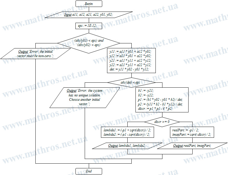
Eigenvalues of a Matrix: From Flowchart to Program Code
If you enjoy programming, try to implement the algorithm for finding the eigenvalues of a matrix using the Krylov method based on the given flowchart in your favorite programming language. It can be Pascal, Python, Java, C++, or any other language.
The main thing is to carefully follow the logic of the algorithm: entering the matrix and the initial vector, checking for possible errors, constructing Krylov vectors, finding the coefficients of the characteristic polynomial, and calculating the eigenvalues.
Such a task will help you not only become familiar with the theory, but also turn it into a practical programming tool.