In numerical methods, eigenvalues and eigenvectors of a matrix help us understand how a square matrix acts on vectors. This topic is important for analyzing linear transformations, studying the stability of processes, and solving many applied problems. So, it is worth starting with the basic definitions first, and only then moving on to the characteristic equation and the method of constructing it through the determinant.
Eigenvalues and Eigenvectors of a Matrix: Basic Concepts
Let a square matrix \( A \) of order \( n \) be given. An eigenvalue of the matrix \( A \) is a number \( \lambda \) for which there exists a nonzero vector \( x \) that satisfies the equation
\[
A\cdot x=\lambda \cdot x.
\]
In this case, the vector \( x \) is called an eigenvector of the matrix \( A \) corresponding to the eigenvalue \( \lambda \). At the same time, the following condition must always hold:
\[
x\neq 0.
\]
Why does the zero vector not work here? Because it does not give us any useful information about the action of the matrix. For any matrix \( A \), the zero vector is transformed into the zero vector. Therefore, it does not show any special property of the matrix.
The meaning of the equality
\[
A\cdot x=\lambda \cdot x
\]
is that the action of the matrix \( A \) on the vector \( x \) comes down to multiplying this vector by the number \( \lambda \). If \( \lambda>0 \), the vector remains directed along the same line. If \( \lambda<0 \), it becomes a vector directed in the opposite direction on the same line. If \( \lambda=0 \), the matrix transforms the corresponding nonzero vector into the zero vector.
So, an eigenvalue shows the numerical result of the matrix action on a certain direction, while an eigenvector defines that direction itself.
Characteristic Equation: From Definition to Computation
Now we need to understand how to move from the definition to actual computations. Let’s start with the main equation:
\[
A\cdot x=\lambda \cdot x.
\]
The left-hand side of this equation already has a matrix form: the matrix \( A \) is multiplied by the vector \( x \). On the right-hand side, the number \( \lambda \) is multiplied by the vector \( x \). To make both sides have the same structure, it is convenient to write the right-hand side using the identity matrix \( E \).
Why can we do this? The identity matrix does not change a vector, that is, \( E\cdot x=x \). Therefore, the product \( \lambda \cdot x \) can be written as
\[
\lambda \cdot x=\lambda\cdot E\cdot x.
\]
So, the original equation takes the form
\[
A\cdot x=\lambda\cdot E\cdot x.
\]
Now let’s move the right-hand side to the left:
\[
A\cdot x-\lambda\cdot E\cdot x=0.
\]
Since both terms contain the vector \( x \), we can factor it out:
\[
(A-\lambda\cdot E)\cdot x=0.
\]
We have obtained a homogeneous system of linear equations. But we are interested not in the zero solution, but in a nonzero solution. When does such a system have a nonzero solution? This is possible when the determinant of its matrix is equal to zero:
\[
\det(A-\lambda\cdot E)=0.
\]
This equation is called the characteristic equation of the matrix \( A \), and the expression
\[
\det(A-\lambda\cdot E)
\]
is called the characteristic determinant.
The roots of the characteristic equation are the eigenvalues of the matrix:
\[
\lambda_1,\lambda_2,\dots,\lambda_n.
\]
However, it is important not to mix up two parts of the process. The characteristic equation gives the eigenvalues, but it does not yet give the eigenvectors themselves. To find the eigenvectors, each eigenvalue \( \lambda_i \) is substituted into the system
\[
(A-\lambda_i \cdot E)\cdot x=0.
\]
The nonzero solutions of this system are the eigenvectors corresponding to the eigenvalue \( \lambda_i \).
Method of Expanding the Characteristic Determinant: Algorithm and Limitations
The obtained equation
\[
\det(A-\lambda\cdot E)=0
\]
must be transformed into an ordinary algebraic equation in terms of \( \lambda \). This is exactly why we expand the characteristic determinant. After expansion, we get a polynomial in \( \lambda \), which is called the characteristic polynomial of the matrix \( A \):
\[
P(\lambda)=\det(A-\lambda\cdot E).
\]
For a square matrix of order \( n \), the characteristic polynomial is a polynomial of degree \( n \) in terms of \( \lambda \). Therefore, the characteristic equation is written as
\[
P(\lambda)=0.
\]
In general form, the characteristic polynomial can be represented by the formula
\[
P(\lambda)=
(-1)^n\cdot
\left(
\lambda^n-\sigma_1\cdot\lambda^{n-1}
+\sigma_2\cdot\lambda^{n-2}
-\dots
+(-1)^n\cdot\sigma_n
\right).
\]
Here, the coefficients \( \sigma_1,\sigma_2,\dots,\sigma_n \) are connected with the principal minors of the matrix \( A \).
For example, the coefficient \( \sigma_1 \) is equal to the sum of the elements on the main diagonal:
\[
\sigma_1=\sum_{\alpha=1}^{n}a_{\alpha\alpha}.
\]
This value is also called the trace of the matrix.
The coefficient \( \sigma_2 \) is equal to the sum of all principal minors of order two:
\[
\sigma_2=
\sum_{\alpha<\beta}
\begin{vmatrix}
a_{\alpha\alpha} & a_{\alpha\beta} \\
a_{\beta\alpha} & a_{\beta\beta}
\end{vmatrix}.
\]
The coefficient \( \sigma_3 \) is equal to the sum of all principal minors of order three:
\[
\sigma_3=
\sum_{\alpha<\beta<\gamma}
\begin{vmatrix}
a_{\alpha\alpha} & a_{\alpha\beta} & a_{\alpha\gamma} \\
a_{\beta\alpha} & a_{\beta\beta} & a_{\beta\gamma} \\
a_{\gamma\alpha} & a_{\gamma\beta} & a_{\gamma\gamma}
\end{vmatrix}.
\]
In the general case, \( \sigma_k \) is the sum of all principal minors of order \( k \). The last coefficient is equal to the determinant of the matrix:
\[
\sigma_n=\det(A).
\]
These formulas show the theoretical structure of the characteristic polynomial. In other words, the coefficients of this polynomial can be connected with the principal minors of the matrix. However, when solving specific problems of order two or three, it is usually easier to work directly: expand the determinant
\[
\det(A-\lambda\cdot E),
\]
combine like terms, and obtain the characteristic equation. This is the approach most often used in practical computations.
The method of expanding the characteristic determinant can be presented as follows:
- Build the matrix \( A-\lambda\cdot E \).
- Find the characteristic determinant \( \det(A-\lambda\cdot E) \).
- Expand this determinant with respect to \( \lambda \) and obtain the characteristic polynomial \( P(\lambda) \).
- Solve the characteristic equation \( P(\lambda)=0 \). Its roots are the eigenvalues of the matrix.
- For each eigenvalue \( \lambda_i \), form the system \( (A-\lambda_i\cdot E)\cdot x=0 \) and find its nonzero solutions. These solutions are the eigenvectors.
So, the method of expanding the characteristic determinant has a clear sequence of steps. It shows the connection between the matrix, the characteristic equation, the eigenvalues, and the eigenvectors. At the same time, this approach is best used for matrices of small order, for example \( 2\times 2 \) or \( 3\times 3 \). For larger matrices, expanding the determinant becomes bulky, so numerical methods often use special algorithms to solve such problems more efficiently.
Eigenvalues and Eigenvectors of a Matrix: Practical Part
In this section, we will apply the sequence described above to specific matrices. Through examples, you will see how the characteristic equation leads to eigenvalues, and how the corresponding homogeneous systems lead to eigenvectors.
Example 1. Find the eigenvalues and eigenvectors of the matrix
\[
A=
\begin{pmatrix}
2 & 1 \\
1 & 2
\end{pmatrix}.
\]
First, let’s write the matrix \( A-\lambda\cdot E \). Since
\[
E=
\begin{pmatrix}
1 & 0 \\
0 & 1
\end{pmatrix},
\]
we get
\[
A-\lambda\cdot E=
\begin{pmatrix}
2-\lambda & 1 \\
1 & 2-\lambda
\end{pmatrix}.
\]
Now let’s form the characteristic equation:
\[
\det(A-\lambda\cdot E)=0.
\]
So,
\[
\begin{vmatrix}
2-\lambda & 1 \\
1 & 2-\lambda
\end{vmatrix}
=0.
\]
Let’s calculate the determinant:
\[
(2-\lambda)\cdot (2-\lambda)-1\cdot 1=0.
\]
That is,
\[
(2-\lambda)^2-1=0.
\]
Now expand the brackets:
\[
4-4\cdot\lambda+\lambda^2-1=0.
\]
After combining like terms, we get
\[
\lambda^2-4\cdot\lambda+3=0.
\]
Let’s factor the quadratic trinomial:
\[
\lambda^2-4\cdot\lambda+3=(\lambda-1)\cdot(\lambda-3).
\]
Therefore,
\[
(\lambda-1)\cdot(\lambda-3)=0.
\]
From here, we get two eigenvalues:
\[
\lambda_1=1,
\qquad
\lambda_2=3.
\]
Now let’s find the eigenvectors.
For the eigenvalue \( \lambda_1=1 \), consider the system
\[
(A-\lambda_1 \cdot E)\cdot x=0.
\]
We have
\[
A-E=
\begin{pmatrix}
1 & 1 \\
1 & 1
\end{pmatrix}.
\]
So,
\[
\begin{pmatrix}
1 & 1 \\
1 & 1
\end{pmatrix}
\cdot
\begin{pmatrix}
x_1 \\
x_2
\end{pmatrix}
=
\begin{pmatrix}
0 \\
0
\end{pmatrix}.
\]
From this, we obtain the equation
\[
x_1+x_2=0.
\]
Therefore, \( x_1=-x_2 \). Let’s choose, for example, \( x_2=1 \). Then \( x_1=-1 \).
So, one of the eigenvectors corresponding to the eigenvalue \( \lambda_1=1 \) has the form
\[
x^{(1)}=
\begin{pmatrix}
-1 \\
1
\end{pmatrix}.
\]
Note (why an eigenvector is not unique). It is worth pausing for a moment here. Why do we say “one of the eigenvectors” and not “the only eigenvector”? The reason is that an eigenvector can be multiplied by any nonzero number, and after that it will still remain an eigenvector for the same eigenvalue.
Indeed, let\[
A\cdot x=\lambda\cdot x,
\]Now multiply the vector \( x \) by some number \( c \), where \( c\neq 0 \). Then, for the vector \( c\cdot x \), we have \( A\cdot (c\cdot x)=c\cdot A \cdot x \). Since \( A\cdot x=\lambda\cdot x \), we can write \( A\cdot (c\cdot x)=c\cdot \lambda\cdot x \). And the right-hand side can be written as \( c\cdot\lambda\cdot x=\lambda\cdot(c\cdot x) \). So,
\[
A\cdot(c\cdot x)=\lambda\cdot(c\cdot x).
\]This means that the vector \( c\cdot x \) is also an eigenvector for the same eigenvalue \( \lambda \).
For example, if
\[
x=
\begin{pmatrix}
-1 \\
1
\end{pmatrix},
\]then the vectors
\[
\begin{pmatrix}
-2 \\
2
\end{pmatrix},
\qquad
\begin{pmatrix}
3 \\
-3
\end{pmatrix},
\qquad
\begin{pmatrix}
-\frac{1}{2} \\
\frac{1}{2}
\end{pmatrix}
\]are also eigenvectors for the same eigenvalue.
Why does this happen? All these vectors lie on the same line. They may have different lengths or point in the opposite direction, but from the point of view of eigenvectors, they describe the same direction of the matrix action. That is why, in problems, it is enough to write one simple nonzero eigenvector.
Now let’s consider the second eigenvalue \( \lambda_2=3 \). We have
\[
A-3\cdot E=
\begin{pmatrix}
-1 & 1 \\
1 & -1
\end{pmatrix}.
\]
Then the system takes the form
\[
\begin{pmatrix}
-1 & 1 \\
1 & -1
\end{pmatrix}
\cdot
\begin{pmatrix}
x_1 \\
x_2
\end{pmatrix}
=
\begin{pmatrix}
0\ \
0
\end{pmatrix}.
\]
From the first row, we get
\[
-x_1+x_2=0.
\]
Hence, \( x_2=x_1 \). Let’s choose \( x_1=1 \). Then \( x_2=1 \).
So, the eigenvector corresponding to the eigenvalue \( \lambda_2=3 \) can be written as
\[
x^{(2)}=
\begin{pmatrix}
1\ \
1
\end{pmatrix}.
\]
Thus, for the given matrix \( A \), we have obtained
\[
\lambda_1=1,
\qquad
x^{(1)}=
\begin{pmatrix}
-1 \\
1
\end{pmatrix},
\\[6pt]
\lambda_2=3,
\qquad
x^{(2)}=
\begin{pmatrix}
1 \\
1
\end{pmatrix}.
\]
Example 2. Find the eigenvalues and eigenvectors of the matrix
\[
A=
\begin{pmatrix}
4 & 2 \\
1 & 3
\end{pmatrix}.
\]
As in the previous example, let’s start with the matrix \( A-\lambda\cdot E \). We have
\[
A-\lambda E=
\begin{pmatrix}
4-\lambda & 2 \\
1 & 3-\lambda
\end{pmatrix}.
\]
Now let’s form the characteristic equation:
\[
\det(A-\lambda\cdot E)=0.
\]
That is,
\[
\begin{vmatrix}
4-\lambda & 2 \\
1 & 3-\lambda
\end{vmatrix}
=0.
\]
Let’s calculate the determinant:
\[
(4-\lambda)\cdot (3-\lambda)-2\cdot 1=0.
\]
Now expand the brackets:
\[
12-4\cdot\lambda-3\cdot\lambda+\lambda^2-2=0.
\]
After simplification, we get
\[
\lambda^2-7\cdot\lambda+10=0.
\]
Let’s factor the quadratic trinomial:
\[
\lambda^2-7\cdot\lambda+10=(\lambda-5)\cdot(\lambda-2).
\]
Therefore,
\[
(\lambda-5)\cdot(\lambda-2)=0.
\]
From here, we obtain the eigenvalues:
\[
\lambda_1=5,
\qquad
\lambda_2=2.
\]
Now let’s find the eigenvectors. For \( \lambda_1=5 \), we have
\[
A-5\cdot E=
\begin{pmatrix}
-1 & 2 \\
1 & -2
\end{pmatrix}.
\]
Then the system has the form
\[
\begin{pmatrix}
-1 & 2 \\
1 & -2
\end{pmatrix}
\cdot
\begin{pmatrix}
x_1 \\
x_2
\end{pmatrix}
=
\begin{pmatrix}
0 \\
0
\end{pmatrix}.
\]
From the first row, we get
\[
-x_1+2\cdot x_2=0.
\]
Hence, \( x_1=2\cdot x_2 \). Let’s choose \( x_2=1 \). Then \( x_1=2 \).
So, an eigenvector for \( \lambda_1=5 \) can be chosen as
\[
x^{(1)}=
\begin{pmatrix}
2 \\
1
\end{pmatrix}.
\]
Now let’s consider \( \lambda_2=2 \). We have
\[
A-2\cdot E=
\begin{pmatrix}
2 & 2 \\
1 & 1
\end{pmatrix}.
\]
So,
\[
\begin{pmatrix}
2 & 2 \\
1 & 1
\end{pmatrix}
\cdot
\begin{pmatrix}
x_1 \\
x_2
\end{pmatrix}
=
\begin{pmatrix}
0 \\
0
\end{pmatrix}.
\]
From the second row, we get
\[
x_1+x_2=0.
\]
Therefore, \( x_1=-x_2 \). Let’s choose \( x_2=1 \). Then \( x_1=-1 \).
So, an eigenvector for \( \lambda_2=2 \) can be written as
\[
x^{(2)}=
\begin{pmatrix}
-1 \\
1
\end{pmatrix}.
\]
Thus, for the given matrix \( A \), we have obtained
\[
\lambda_1=5,
\qquad
x^{(1)}=
\begin{pmatrix}
2 \\
1
\end{pmatrix},
\\[6pt]
\lambda_2=2,
\qquad
x^{(2)}=
\begin{pmatrix}
-1 \\
1
\end{pmatrix}.
\]
Example 3. Find the eigenvalues and eigenvectors of the matrix
\[
A=
\begin{pmatrix}
2 & 1 & 0 \\
0 & 3 & 0 \\
0 & 0 & 4
\end{pmatrix}.
\]
In this example, we have a triangular matrix. Therefore, the characteristic determinant is much easier to calculate than for an arbitrary matrix of order three. If all elements below the main diagonal were not equal to zero, we would have to fully expand a third-order determinant and perform more intermediate transformations.
Let’s write
\[
A-\lambda\cdot E=
\begin{pmatrix}
2-\lambda & 1 & 0 \\
0 & 3-\lambda & 0 \\
0 & 0 & 4-\lambda
\end{pmatrix}.
\]
The characteristic equation has the form
\[
\det(A-\lambda\cdot E)=0.
\]
That is,
\[
\begin{vmatrix}
2-\lambda & 1 & 0 \\
0 & 3-\lambda & 0 \\
0 & 0 & 4-\lambda
\end{vmatrix}
=0.
\]
Since the matrix is triangular, its determinant is equal to the product of the elements on the main diagonal:
\[
(2-\lambda)\cdot(3-\lambda)\cdot(4-\lambda)=0.
\]
From here, we immediately obtain the eigenvalues:
\[
\lambda_1=2,
\qquad
\lambda_2=3,
\qquad
\lambda_3=4.
\]
Now let’s find the eigenvectors. For \( \lambda_1=2 \), we have
\[
A-2\cdot E=
\begin{pmatrix}
0 & 1 & 0 \\
0 & 1 & 0 \\
0 & 0 & 2
\end{pmatrix}.
\]
Then
\[
\begin{pmatrix}
0 & 1 & 0 \\
0 & 1 & 0 \\
0 & 0 & 2
\end{pmatrix}
\cdot
\begin{pmatrix}
x_1 \\
x_2 \\
x_3
\end{pmatrix}
=
\begin{pmatrix}
0 \\
0 \\
0
\end{pmatrix}.
\]
From this system, we get
\[
x_2=0,
\qquad
x_3=0.
\]
The variable \( x_1 \) remains free. Let’s choose \( x_1=1 \). Then an eigenvector for \( \lambda_1=2 \) can be written as
\[
x^{(1)}=
\begin{pmatrix}
1 \\
0 \\
0
\end{pmatrix}.
\]
For \( \lambda_2=3 \), we get
\[
A-3\cdot E=
\begin{pmatrix}
-1 & 1 & 0 \\
0 & 0 & 0 \\
0 & 0 & 1
\end{pmatrix}.
\]
So,
\[
\begin{pmatrix}
-1 & 1 & 0 \\
0 & 0 & 0 \\
0 & 0 & 1
\end{pmatrix}
\cdot
\begin{pmatrix}
x_1 \\
x_2 \\
x_3
\end{pmatrix}
=
\begin{pmatrix}
0 \\
0 \\
0
\end{pmatrix}.
\]
From the first row, we have
\[
-x_1+x_2=0.
\]
That is, \( x_2=x_1 \). From the third row, we get \( x_3=0 \). Let’s choose \( x_1=1 \). Then
\[
x_2=1,
\qquad
x_3=0.
\]
So, an eigenvector for \( \lambda_2=3 \) has the form
\[
x^{(2)}=
\begin{pmatrix}
1 \\
1 \\
0
\end{pmatrix}.
\]
Finally, let’s consider \( \lambda_3=4 \). We have
\[
A-4\cdot E=
\begin{pmatrix}
-2 & 1 & 0 \\
0 & -1 & 0 \\
0 & 0 & 0
\end{pmatrix}.
\]
Then
\[
\begin{pmatrix}
-2 & 1 & 0 \\
0 & -1 & 0 \\
0 & 0 & 0
\end{pmatrix}
\cdot
\begin{pmatrix}
x_1 \\
x_2 \\
x_3
\end{pmatrix}
=
\begin{pmatrix}
0 \\
0 \\
0
\end{pmatrix}.
\]
From the second row, we have \( -x_2=0 \). Therefore, \( x_2=0 \). Substitute this into the first row:
\[
-2\cdot x_1+x_2=0.
\]
Since \( x_2=0 \), we get \( -2\cdot x_1=0 \). Hence, \( x_1=0 \).
The variable \( x_3 \) remains free. Let’s choose \( x_3=1 \). So, an eigenvector for \( \lambda_3=4 \) can be written as
\[
x^{(3)}=
\begin{pmatrix}
0 \\
0 \\
1
\end{pmatrix}.
\]
Thus, for the given matrix \( A \), we have
\[
\lambda_1=2,
\qquad
x^{(1)}=
\begin{pmatrix}
1 \\
0 \\
0
\end{pmatrix},
\\[6pt]
\lambda_2=3,
\qquad
x^{(2)}=
\begin{pmatrix}
1 \\
1 \\
0
\end{pmatrix},
\\[6pt]
\lambda_3=4,
\qquad
x^{(3)}=
\begin{pmatrix}
0 \\
0 \\
1
\end{pmatrix}.
\]
What to Study Next: Methods for Continuing the Topic
After the method of expanding the characteristic determinant, it is worth moving on to special methods for finding eigenvalues. They show how to work with matrices of larger order and how to organize computations more effectively.
- Danilevsky Method: Transition to the Characteristic Polynomial — The article will explain how the Danilevsky method transforms a matrix and helps obtain its characteristic polynomial.
- Krylov Method: Constructing Equations for Eigenvalues — This material will discuss how the Krylov method forms a system of equations and helps find the characteristic polynomial of a matrix.
- Leverrier Method: Computing Polynomial Coefficients — The article will show how the Leverrier method finds the coefficients of the characteristic polynomial through consecutive matrix computations.
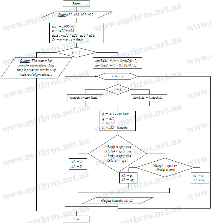
Eigenvalues and Eigenvectors of a Matrix in Programming: Create Your Own Method Implementation
If you are interested not only in reading about the method but also in testing it in code, take a look at the flowchart below. It can become the basis for a small program in your favorite programming language that finds the eigenvalues and eigenvectors of a matrix by expanding the characteristic polynomial.
This kind of work will help you better see the connection between the matrix, the characteristic equation, and the program logic. Also, it is a good way to check how the theoretical algorithm behaves for different matrices of small order.