Newton’s method is one of the classical numerical methods used to find the minimum of a function of one variable. This topic matters because, in practice, the minimum value cannot always be found by simple transformations. That is why iterative methods are used, since they allow us to move step by step toward the desired point.
In this article, we will look step by step at the main idea of the method, derive the iterative formula, determine when the calculations should stop, and then apply this approach to a specific problem. This structure makes it easier not only to see the final formula, but also to understand exactly how it works.
Newton’s Method for Minimization: How the Local Approximation Is Built
Suppose we are given a function \( f(x) \) for which we need to find a point of local minimum. In Newton’s method, we do not gradually narrow an interval as in interval methods. Instead, we choose an initial approximation \( x_0 \), and then build a sequence of points
\[
x_0, x_1, x_2, x_3, \dots
\]
that should lead us to the desired minimum point.
The idea behind this approach is that near the current point \( x_k \), we replace the function with a simpler expression. For this, we use the second-order Taylor expansion. So, in a neighborhood of the point \( x_k \), we have the approximation
\[
f(x_k+t) \approx f(x_k) + f’(x_k)\cdot t + \frac{1}{2}\cdot f’’(x_k)\cdot t^2,
\]
where \( t \) denotes the increment from the current approximation.
So, instead of working directly with the function \( f(x) \) at each step, we work with its local quadratic approximation. This is an important point: at each iteration, Newton’s method minimizes not the original function itself, but this approximate quadratic model.
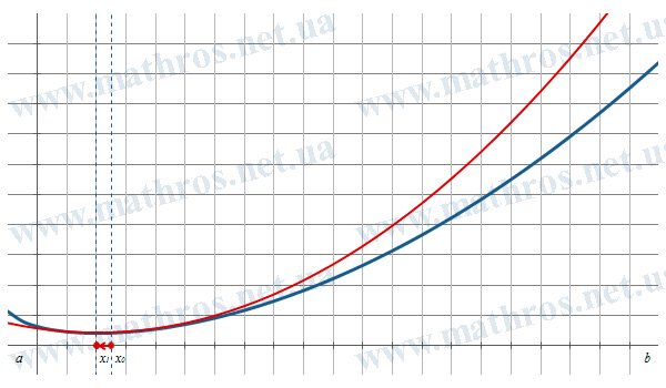
This approach works when the function is sufficiently smooth. In other words, in the region we are interested in, it must have at least the first and second derivatives. In addition, the second derivative at the current point must not be equal to zero. Otherwise, the transition to the next approximation cannot be written in the required form.
Deriving the Formula of Newton’s Method: How the Next Approximation Is Obtained
Now let us move from the general idea to the actual formula. Let us denote the local quadratic approximation by
\[
\varphi(t)=f(x_k) + f’(x_k)\cdot t + \frac{1}{2}\cdot f’’(x_k)\cdot t^2.
\]
It is exactly the function \( \varphi(t) \) that must be minimized with respect to the variable \( t \). To do this, we set its derivative equal to zero:
\[
\varphi’(t)=0.
\]
Now let us compute the derivative:
\[
\varphi’(t)=f’(x_k)+f’’(x_k)\cdot t.
\]
So we obtain the equation
\[
f’(x_k)+f’’(x_k)\cdot t=0.
\]
From this, we find the step size:
\[
f’’(x_k)\cdot t=-f’(x_k),
\qquad
t=-\frac{f’(x_k)}{f’’(x_k)}.
\]
Since the new point is defined by the relation
\[
x_{k+1}=x_k+t,
\]
after substitution, we get the main iterative formula of Newton’s method:
\[
x_{k+1}=x_k-\frac{f’(x_k)}{f’’(x_k)}.
\]
This is exactly the formula used in practical calculations. It shows how to move from the current approximation \( x_k \) to the new approximation \( x_{k+1} \).
Here, it is important to notice one more thing. If at some minimum point \( x_{\min} \) the following conditions hold:
\[
f’(x_{\min})=0,
\qquad
f’’(x_{\min})>0,
\]
then we are dealing with a local minimum. The first condition gives a stationary point, while the second confirms that this point corresponds to a minimum rather than a maximum.
At the same time, it is worth remembering that the method is sensitive to the choice of the initial approximation \( x_0 \). If the starting point is chosen well, convergence can be very fast. If not, the process may slow down or lead to a different stationary point.
Stopping Criterion for the Iterations: How to Determine the Final Result
After deriving the iterative formula, a natural question appears: when exactly should the calculations stop? In practice, the iterative process is not continued indefinitely. Instead, it is stopped when the required accuracy has been reached.
Most often, the following condition is used:
\[
|x_{k+1}-x_k|<\varepsilon,
\]
where \( \varepsilon>0 \) is a predefined accuracy level. In this case, we check how close two neighboring approximations have become. If the difference between them is already small, we assume that the sequence of approximations has essentially stabilized. So here, \( \varepsilon \) controls the closeness of neighboring approximations in terms of the variable \( x \), not directly the error in the function value.
Sometimes, another criterion is also used:
\[
|f’(x_k)|<\varepsilon.
\]
Here, we check whether the value of the first derivative has become sufficiently small. This means that the current point is already close to a stationary point.
Also, in practical computations, it is common to set a maximum number of iterations. This is done so that the algorithm does not run for too long in cases of slow convergence or an unfortunate choice of the initial point.
If the stopping condition is satisfied, then the last approximation obtained is taken as the approximate value of the minimum point. So, after the iterations are completed, we write
\[
x^*\approx x_{k+1}.
\]
After that, we calculate the approximate minimum value of the function:
\[
f_{\min}\approx f(x^*).
\]
Practical Part: How Newton’s Method Works on a Specific Problem
Now we can move on to an example. The theoretical formulas have already been derived, so now it is time to see how they work in practice. A specific problem clearly shows the role of the derivatives, the sequence of iterations, and the check of the accuracy condition.
Example 1. Find the minimum value of the function \( f(x)=x^4-4 \cdot x^2+5 \) on the interval \( [1,2] \) with accuracy \( \varepsilon=0.05 \), using Newton’s method
Let us consider the function \( f(x)=x^4-4 \cdot x^2+5 \) on the interval \( [1,2] \). On this interval, it is sufficiently smooth, which means it has both the first and second derivatives. Let us take the initial approximation \( x_0=1.5 \), since it belongs to the given interval. In addition, it is located near the minimum point, so it is a convenient starting point for the iterative process.
![Graph of the function f(x)=x^4-4*x^2+5 on the interval [1,2]](https://www.mathros.net.ua/en/wp-content/uploads/2026/04/xnewtons-method-minimum-of-a-function2.jpg.pagespeed.ic.T13hcFYx_C.jpg)
First, let us find the derivatives:
\[
f’(x)=4\cdot x^3-8\cdot x,
\qquad
f’’(x)=12\cdot x^2-8.
\]
For the first iteration, we calculate the values of the derivatives at the point \( x_0=1.5 \):
\[
\begin{gathered}
f’(1.5)=4\cdot(1.5)^3-8\cdot1.5=13.5-12=1.5,
\\[6pt]
f’’(1.5)=12\cdot(1.5)^2-8=27-8=19.
\end{gathered}
\]
This gives the new approximation
\[
x_1=x_0-\frac{f’(x_0)}{f’’(x_0)}=1.5-\frac{1.5}{19}\approx 1.421.
\]
For the second iteration, we take the point \( x_1\approx 1.421 \):
\[
\begin{gathered}
f’(1.421)=4\cdot(1.421)^3-8\cdot1.421\approx 0.337,
\\[6pt]
f’’(1.421)=12\cdot(1.421)^2-8\approx 16.234.
\end{gathered}
\]
So,
\[
x_2=x_1-\frac{f’(x_1)}{f’’(x_1)}\approx 1.421-\frac{0.337}{16.234}\approx 1.4.
\]
Now we check the accuracy condition:
\[
|x_2-x_1|=|1.4-1.421|=0.021.
\]
Since \( 0.021<0.05 \), the iterative process can be stopped at this stage.
The last approximation obtained is \( x_2 \), so we take it as the approximate value of the minimum point:
\[
x^*\approx x_2\approx 1.4.
\]
Next, we calculate the approximate minimum value of the function:
\[
f_{\min}\approx f(x^*)=f(1.4).
\]
Substituting the approximate value, we get:
\[
f(1.4)=(1.4)^4-4 \cdot (1.4)^2+5.
\]
Now compute the powers:
\[
1.4^2=1.96,
\qquad
1.4^4=(1.96)^2=3.8416.
\]
Therefore,
\[
f(1.4)=3.8416-4\cdot1.96+5=3.8416-7.84+5=1.0016.
\]
So, by Newton’s method, we obtain
\[
x^*\approx 1.4,
\qquad
f_{\min}\approx 1.0016.
\]
This result agrees well with the exact solution, because for the function \( f(x)=x^4-4 \cdot x^2+5 \) on the interval \( [1,2] \), the minimum is reached at \( x=\sqrt{2} \), and the corresponding smallest value is \( f(\sqrt{2})=1 \).
So, this corrected example shows the proper application of Newton’s method: from choosing the initial point and calculating the derivatives to checking the stopping condition at the right step and finding the approximate minimum value of the function.
What to Explore Next: Related Topics in Optimization
We have now gone through Newton’s method for a function of one variable in a clear and consistent way. But where should you go next? A logical next step is to look at directions in which the search for a minimum is studied for functions of several variables and in a slightly different format.
- Newton’s Method for Several Variables: How the Search for a Minimum Changes — This topic explains how Newton’s method extends to functions of several variables and what changes when we look for a minimum in that setting.
- Coordinate Descent: How Alternating Search Works — Here, you will see an approach in which the minimum is found step by step with respect to each variable, making the calculation process easier to understand.
- Gradient Descent: How the Direction of Decrease Is Chosen — This article focuses on a way to find the minimum of a function of several variables by choosing the direction in which the function value decreases.
Newton’s Method in Programming: Try Implementing the Algorithm Yourself
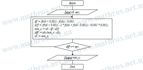
The flowchart below can become more than just an addition to the theoretical material. It can also serve as a convenient basis for your own practical work. Why not use it as a starting point and create a small program in your favorite programming language for finding the minimum value of a function using Newton’s method?
This approach helps you see how a mathematical idea turns into a step-by-step algorithm and then into clear, understandable code. It is also a good opportunity to test the method on different functions and get a much better feel for how it works in real practice.