The dichotomous search method is one of the basic numerical methods used to find the minimum of a function of one variable on a given interval. Why is this approach worth studying on its own? First, because it provides a clear sequence of steps and shows how a minimization problem can be solved step by step. It is also especially useful for learning, since it makes it easy to see how the search interval gradually becomes smaller. That is why, in what follows, we will examine the main conditions for applying this method and the principle of constructing successive approximations to the minimum point.
Dichotomous Search Method: Conditions of Use and the Main Idea
Suppose we are given a function \( f(x) \) and need to find its minimum point on the interval \( [a_0,b_0] \). Here, one important condition should be stated right away: the function must be unimodal on this interval. What does that mean in this context? It means that on the interval \( [a_0,b_0] \), there is only one point at which the function reaches its smallest value. Only under this condition can we repeatedly discard parts of the interval without losing the desired minimum.
Next, we choose the search accuracy \( \varepsilon \). This shows how narrow the final interval should be, within which the minimum point lies. It is also helpful to distinguish between two ideas here. First, there is the minimum point \( x^* \). Second, there is the minimum value of the function \( f(x^*) \). The dichotomous search method mainly helps us approximately determine the point \( x^* \), and then, if necessary, we calculate the value of the function at that point. So, the goal here is not to find the exact solution in closed form, but rather to obtain an approximate result with a given accuracy.
On the initial interval \( [a_0,b_0] \), two internal points are constructed:
\[
x_1^{(0)}=\frac{a_0+b_0-\delta}{2}, \qquad x_2^{(0)}=\frac{a_0+b_0+\delta}{2},
\]
where \( \delta \) is a small positive number satisfying the condition
\[
0<\delta<\varepsilon.
\]
Why do we need exactly two points? Because a single value at the midpoint is not enough to determine in which direction the interval should be narrowed. However, comparing the function values at two nearby internal points gives us the information we need. The parameter \( \delta \) is introduced so that the points \( x_1^{(0)} \) and \( x_2^{(0)} \) do not coincide with the midpoint of the interval, but instead lie very close to it on opposite sides. The rest of the search procedure is based on this idea.
So, at the first step, we still do not obtain the final answer. Instead, we create the basis for comparing function values and continuing the method. Only after this can we move on to the successive narrowing of the search interval.
Successive Narrowing of the Interval: How New Approximations Are Obtained
Now let us move to the next stage. After constructing the points \( x_1^{(0)} \) and \( x_2^{(0)} \), we calculate the values of the function at these points, \( f \left(x_1^{(0)}\right) \) and \( f \left(x_2^{(0)}\right) \).
Next, we compare these values. This comparison shows which part of the current interval can be discarded.
- If \( f \left(x_1^{(0)}\right)<f \left(x_2^{(0)}\right) \), then the minimum should be sought on the interval \( [a_1,b_1]=[a_0,x_2^{(0)}] \).
- If \( f \left(x_1^{(0)}\right)>f \left(x_2^{(0)}\right) \), then the new search interval becomes \( [a_1,b_1]=[x_1^{(0)},b_0] \).
- If the values are equal, that is, \( f \left(x_1^{(0)}\right)=f \left(x_2^{(0)}\right) \), then the minimum point lies between these two points, so we take the interval \( [a_1,b_1]=[x_1^{(0)},x_2^{(0)}] \).
So, after the first comparison, we already obtain a new, narrower search interval. This is the practical purpose of each iteration: not to find the minimum point immediately, but to narrow the region containing it step by step. By the way, the case \( f \left(x_1^{(0)}\right)=f \left(x_2^{(0)}\right) \) occurs less often in practice, but it is still important to include it as part of the full description of the algorithm.
After that, the process is repeated for the new interval \( [a_1,b_1] \). For this interval, two internal points are again constructed:
\[
x_1^{(1)}=\frac{a_1+b_1-\delta}{2}, \qquad x_2^{(1)}=\frac{a_1+b_1+\delta}{2},
\]
then the values \( f \left(x_1^{(1)}\right) \) and \( f \left(x_2^{(1)}\right) \) are found, and the interval is narrowed once again.
In the same way, at an arbitrary \( k \)-th iteration, when we already have the interval \( [a_k,b_k] \), the internal points are calculated using the formulas
\[
x_1^{(k)}=\frac{a_k+b_k-\delta}{2}, \qquad x_2^{(k)}=\frac{a_k+b_k+\delta}{2}.
\]
After comparing the values \( f \left(x_1^{(k)}\right) \) and \( f \left(x_2^{(k)}\right) \), we obtain a new interval \( [a_{k+1},b_{k+1}] \). In this way, with each iteration, the search region becomes smaller. Is it not convenient when a complicated problem is reduced to repeating just a few clear steps?
The process continues until the length of the current interval becomes smaller than the given accuracy:
\[
b_k-a_k<\varepsilon.
\]
After that, the minimum point is considered to have been found approximately. As an approximate value of this point, the midpoint of the final interval is often taken:
\[
x^*\approx \frac{a_k+b_k}{2}.
\]
If it is also necessary to specify the minimum value of the function, then \( f(x^*) \) is calculated as well.
Thus, the dichotomous search method allows us not to look for the exact solution in closed form, but to approach it step by step with a predetermined accuracy. That is why this approach is an important part of the topic of numerical minimization of a function of one variable.
Practical Part: How the Dichotomous Search Method Works on a Specific Problem
Now let us move on to the practical part. The theoretical scheme is already clear, but how does it actually work in real calculations? A simple example makes it easy to see how the dichotomous search method gradually narrows the search interval and brings us closer to the minimum value of the function.
Example 1. Find the minimum value of the function \( f(x)=(x-2)^2+1 \) on the interval \( [1,4] \) with accuracy \( \varepsilon=0.1 \), using the dichotomous search method
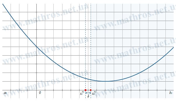
Let us consider the function \( f(x)=(x-2)^2+1 \) on the interval \( [1,4] \). On this interval, it is unimodal, since it has only one minimum point at \( x=2 \). Therefore, the dichotomous search method can be applied correctly here.
![Graph of the function f(x)=(x-2)^2+1 on the interval [1,4]](https://www.mathros.net.ua/en/wp-content/uploads/2026/04/xdichotomous-search-method2.jpg.pagespeed.ic.RzHsBM0jC9.jpg)
We start with the initial interval
\[
[a_0,b_0]=[1,4].
\]
Let us take \( \delta=0.05 \), since this number is smaller than the given accuracy \( \varepsilon=0.1 \).
For the first iteration, we calculate two internal points:
\[
\begin{gathered}
x_1^{(0)}=\frac{a_0+b_0-\delta}{2}=\frac{1+4-0.05}{2}=2.475,
\\[6pt]
x_2^{(0)}=\frac{a_0+b_0+\delta}{2}=\frac{1+4+0.05}{2}=2.525.
\end{gathered}
\]
Now let us find the values of the function at these points:
\[
\begin{gathered}
f\left(x_1^{(0)}\right)=f(2.475)=(2.475-2)^2+1=1.226,
\\[6pt]
f\left(x_2^{(0)}\right)=f(2.525)=(2.525-2)^2+1=1.276.
\end{gathered}
\]
Since \( f\left(x_1^{(0)}\right)<f\left(x_2^{(0)}\right) \), we take the new search interval
\[
[a_1,b_1]=[a_0,x_2^{(0)}]=[1,2.525].
\]
Now we move to the second iteration. For the interval \( [a_1,b_1]=[1,2.525] \), we have
\[
\begin{gathered}
x_1^{(1)}=\frac{a_1+b_1-\delta}{2}=\frac{1+2.525-0.05}{2}=1.738,
\\[6pt]
x_2^{(1)}=\frac{a_1+b_1+\delta}{2}=\frac{1+2.525+0.05}{2}=1.788.
\end{gathered}
\]
We calculate the function values:
\[
\begin{gathered}
f\left(x_1^{(1)}\right)=f(1.738)=(1.738-2)^2+1=1.069,
\\[6pt]
f\left(x_2^{(1)}\right)=f(1.788)=(1.788-2)^2+1=1.045.
\end{gathered}
\]
Here we get \( f\left(x_1^{(1)}\right)>f\left(x_2^{(1)}\right) \), so the new interval becomes
\[
[a_2,b_2]=[x_1^{(1)},b_1]=[1.738,2.525].
\]
At the third iteration, we find
\[
\begin{gathered}
x_1^{(2)}=\frac{a_2+b_2-\delta}{2}=\frac{1.738+2.525-0.05}{2}=2.107,
\\[6pt]
x_2^{(2)}=\frac{a_2+b_2+\delta}{2}=\frac{1.738+2.525+0.05}{2}=2.157.
\end{gathered}
\]
Then
\[
\begin{gathered}
f\left(x_1^{(2)}\right)=f(2.107)=(2.107-2)^2+1=1.011,
\\[6pt]
f\left(x_2^{(2)}\right)=f(2.157)=(2.157-2)^2+1=1.025.
\end{gathered}
\]
Since \( f\left(x_1^{(2)}\right)<f\left(x_2^{(2)}\right) \), we narrow the interval to
\[
[a_3,b_3]=[a_2,x_2^{(2)}]=[1.738,2.157].
\]
Next, we repeat the same procedure again. For the interval \( [a_3,b_3]=[1.738,2.157] \), we have
\[
\begin{gathered}
x_1^{(3)}=\frac{a_3+b_3-\delta}{2}=\frac{1.738+2.157-0.05}{2}=1.923,
\\[6pt]
x_2^{(3)}=\frac{a_3+b_3+\delta}{2}=\frac{1.738+2.157+0.05}{2}=1.973.
\end{gathered}
\]
The function values are
\[
\begin{gathered}
f\left(x_1^{(3)}\right)=f(1.923)=(1.923-2)^2+1=1.006,
\\[6pt]
f\left(x_2^{(3)}\right)=f(1.973)=(1.973-2)^2+1=1.001.
\end{gathered}
\]
Now \( f\left(x_1^{(3)}\right)>f\left(x_2^{(3)}\right) \), so the new search interval is
\[
[a_4,b_4]=[x_1^{(3)},b_3]=[1.923,2.157].
\]
Let us perform the calculations once again. For the interval \( [a_4,b_4]=[1.923,2.157] \), we get
\[
\begin{gathered}
x_1^{(4)}=\frac{a_4+b_4-\delta}{2}=\frac{1.923+2.157-0.05}{2}=2.015,
\\[6pt]
x_2^{(4)}=\frac{a_4+b_4+\delta}{2}=\frac{1.923+2.157+0.05}{2}=2.04.
\end{gathered}
\]
We calculate the function values:
\[
\begin{gathered}
f\left(x_1^{(4)}\right)=f(2.015)=(2.015-2)^2+1=1,
\\[6pt]
f\left(x_2^{(4)}\right)=f(2.04)=(2.04-2)^2+1=1.002.
\end{gathered}
\]
Since \( f\left(x_1^{(4)}\right)<f\left(x_2^{(4)}\right) \), we obtain the new interval
\[
[a_5,b_5]=[a_4,x_2^{(4)}]=[1.923,2.04].
\]
Its length is
\[
b_5-a_5=2.04-1.923=0.117,
\]
so the accuracy condition is not yet satisfied, and we need to make one more step.
For the interval \( [a_5,b_5]=[1.923,2.04] \), we have
\[
\begin{gathered}
x_1^{(5)}=\frac{a_5+b_5-\delta}{2}=\frac{1.923+2.04-0.05}{2}=1.957,
\\[6pt]
x_2^{(5)}=\frac{a_5+b_5+\delta}{2}=\frac{1.923+2.04+0.05}{2}=2.007.
\end{gathered}
\]
Then
\[
\begin{gathered}
f\left(x_1^{(5)}\right)=f(1.957)=(1.957-2)^2+1=1.002,
\\[6pt]
f\left(x_2^{(5)}\right)=f(2.007)=(2.007-2)^2+1=1.
\end{gathered}
\]
We can see that \( f\left(x_1^{(5)}\right)>f\left(x_2^{(5)}\right) \), so the new search interval is
\[
[a_6,b_6]=[x_1^{(5)},b_5]=[1.957,2.04].
\]
Now let us check its length:
\[
b_6-a_6=2.04-1.957=0.083<0.1.
\]
So, the accuracy condition is satisfied. As the approximate value of the minimum point, we take the midpoint of the final interval:
\[
x^*\approx \frac{a_6+b_6}{2}=\frac{1.957+2.04}{2}=1.999.
\]
Then the approximate minimum value of the function is
\[
f_{\min}\approx f(x^*)=f(1.999)=(1.999-2)^2+1=1.
\]
So, using the dichotomous search method, we obtain
\[
x^*\approx 1.999,
\qquad
f_{\min}\approx 1.
\]
This result agrees very well with the exact answer, because for the function \( f(x)=(x-2)^2+1 \), the minimum is indeed reached at \( x=2 \), and the smallest value is \( 1 \). Thus, this practical example clearly shows how the dichotomous search method, through successive narrowing of the interval, makes it possible to approximately determine the minimum value of a function.
Additional Topics: Where to Go Next
Now that the main idea of the dichotomous search method has become clearer, it is a good time to look at other approaches to minimization as well. What should you read next? Below are several topics that continue the study of numerical methods in a logical and useful way.
- Newton’s Method: How to Take the Behavior of a Function into Account — This article discusses how to find a minimum using derivatives and why this approach often gives fast results.
- Coordinate Descent: How to Search for a Minimum One Variable at a Time — This article shows how the minimum of a function of several variables can be found by changing each coordinate step by step.
- Gradient Descent: How to Move in the Direction of Decreasing Function Values — This article examines one of the best-known minimization methods for functions of several variables and explains its main idea.
Dichotomous Search Method in Code: Create Your Own Program for Finding a Minimum
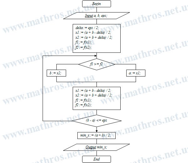
Now look at the flowchart below not only as an illustration, but also as a ready foundation for a small learning project. Why not use it and write a small program in your favorite programming language that determines the minimum value of a unimodal function using the dichotomous search method? This kind of work clearly shows how a mathematical idea turns into an understandable algorithm, and then into program code that can be tested on different examples. In addition, it is a good opportunity to understand the method better not only in theory, but also through practical implementation.