Fibonacci Method: From the Main Idea to a Practical Example

The Fibonacci method is one of the classical numerical methods used to find the minimum of a function of one variable on a given interval. It is valued because it narrows the search interval step by step while also making efficient use of calculations that have already been performed. Why is this important? Because in optimization problems, it is not always convenient to find an exact solution in explicit form. For this reason, in practice, we often look not for an exact answer, but for a sufficiently accurate approximation.

In this article, we will examine what problem the Fibonacci method solves, why Fibonacci numbers are used in it, how the interior points are constructed, and how an approximate value of the minimum point is obtained at the end.

Fibonacci Method: What Problem Does This Approach Solve?

Let us begin with the problem statement. Suppose we are given a function

\[
f(x), \qquad x \in [a,b].
\]

We need to find a point \( x^* \) on the interval \( [a,b] \) at which the function attains its smallest value:

\[
f(x^*)=\min_{x\in[a,b]} f(x).
\]

In other words, we are looking for the minimum of a function on a given interval. But how can we do this without checking a large number of points? This is exactly where one-dimensional optimization methods are used. In particular, the Fibonacci method allows us to avoid testing values randomly and instead narrow the interval step by step, keeping only the part that contains the minimum point.

At the same time, we should remember an important condition. Usually, the Fibonacci method is applied to a unimodal function on the interval \( [a,b] \). This means that the function has only one minimum on that interval. In practical terms, this can be understood as follows: before the minimum point, the function values decrease, and after it, they increase. Why is this condition so important? Because it is exactly what allows us to correctly discard part of the interval after comparing the function values at two interior points.

So, the main idea of the method is simple: we do not try to find the exact minimum point immediately. Instead, we gradually reduce the search region until we obtain a sufficiently small interval. It is this interval that shows where the required minimum is located.

Fibonacci Numbers: Why the Fibonacci Method Relies on Them

At this point, a very natural question arises: why does this method use Fibonacci numbers in particular? The reason is that they make it possible to organize the gradual narrowing of the interval in a very convenient way. Because of this, after each step, one of the points that has already been found can be reused, so we do not need to calculate the function values at both points again every time.

The sequence of Fibonacci numbers is defined recursively:

\[
\begin{gathered}
F_1=1,\qquad F_2=1,
\\[4pt]
F_k=F_{k-1}+F_{k-2}, \qquad k>2.
\end{gathered}
\]

Its first few terms are:

\[
F_3=2,\quad F_4=3,\quad F_5=5,\quad F_6=8,\quad F_7=13,\quad F_8=21,\dots
\]

These are exactly the numbers used to choose the positions of the interior points on the current interval. In addition, they help connect the length of the initial interval with the required search accuracy.

Let \( \varepsilon \) be the given error tolerance. Then we choose the smallest number \( F_n \) for which the inequality

\[
F_n \geq \frac{b-a}{\varepsilon}
\]

holds.

What does this condition mean? It allows us to determine in advance how many steps are needed for the search interval to become sufficiently small. So, the number of iterations in the Fibonacci method is not random. On the contrary, it is determined beforehand by the length of the initial interval and the required accuracy.

It is also useful to notice one more important point here. If we want to obtain a more accurate result, that is, if we take a smaller \( \varepsilon \), then the value

\[
\frac{b-a}{\varepsilon}
\]

becomes larger. This means that we need to take a larger Fibonacci number and, accordingly, perform more steps. So, in this method, the accuracy and the number of iterations are directly connected.

Initial Interval: How the Interior Points Are Calculated

After the required number \( F_n \) has been chosen, we can move on to constructing two interior points on the interval \( [a_0,b_0]=[a,b] \). It is at these points that the function values are calculated at the first step.

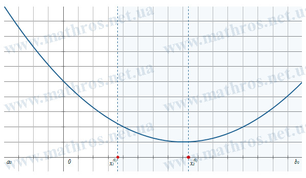
The points \( x_1^{(0)} ) and ( x_2^{(0)} \) are defined by the formulas

\[
x_1^{(0)}=a_0+\frac{F_{n-2}}{F_n}\cdot (b_0-a_0), \qquad
x_2^{(0)}=a_0+\frac{F_{n-1}}{F_n}\cdot (b_0-a_0).
\]

These points lie inside the interval \( [a_0,b_0] \), and they are arranged in the following order:

\[
a_0<x_1^{(0)}<x_2^{(0)}<b_0.
\]

Why is it important to emphasize this? Because later, it is exactly the order of the points that allows us to correctly determine which part of the interval can be discarded after comparing the function values.

Next, we calculate \( f\left(x_1^{(0)}\right) \) and \( f\left(x_2^{(0)}\right) \), and then compare the obtained values. If \( f\left(x_1^{(0)}\right)\leq f\left(x_2^{(0)}\right) \), then, under the unimodality condition, this means that the minimum point does not lie to the right of \( x_2^{(0)} \). Therefore, the right part of the interval can be discarded, and the new search interval takes the form \( [a_1,b_1]=[a_0,x_2^{(0)}] \).

If, on the other hand, \( f\left(x_1^{(0)}\right)>f\left(x_2^{(0)}\right) \), then the minimum point does not lie to the left of \( x_1^{(0)} \). In that case, the left part is discarded, and the new interval becomes \( [a_1,b_1]=[x_1^{(0)},b_0] \).

So, after each comparison, the length of the interval decreases. Even at this stage, it is easy to see how the method gradually isolates the region in which the minimum point is located.

Fibonacci Method: How the Search Interval Is Narrowed Step by Step

After the first comparison, the process does not stop. On the contrary, the Fibonacci method repeats the same actions on the new, already narrower interval. However, there is an important advantage here: one of the interior points does not need to be constructed again, because it is carried over from the previous step. This is exactly why the method works efficiently.

If \( f\left(x_1^{(0)}\right)\leq f\left(x_2^{(0)}\right) \), then we set

\[
a_1=a_0, \qquad b_1=x_2^{(0)}, \qquad x_2^{(1)}=x_1^{(0)},
\]

and the new point \( x_1^{(1)} \) is calculated by the formula

\[
x_1^{(1)}=a_1+\frac{F_{n-3}}{F_{n-1}}\cdot (b_1-a_1).
\]

If, on the other hand, \( f\left(x_1^{(0)}\right)>f\left(x_2^{(0)}\right) \), then we take

\[
a_1=x_1^{(0)}, \qquad b_1=b_0, \qquad x_1^{(1)}=x_2^{(0)},
\]

and the new point \( x_2^{(1)} \) is found as follows:

\[
x_2^{(1)}=a_1+\frac{F_{n-2}}{F_{n-1}}\cdot (b_1-a_1).
\]

After that, we calculate the function value only at the new point and perform the next comparison. Then the procedure is repeated step by step. In this way, the interval of uncertainty becomes smaller each time.

What do we obtain as a result? Not an exact analytical solution, but a sufficiently narrow interval inside which the minimum point is located. That is why the Fibonacci method belongs to numerical methods of approximate search.

After the algorithm is completed, a natural question appears: which exact point should be taken as the approximate value of the minimum point? Since at the end we have a small interval \( [a_k,b_k] \) that contains the required point, in practice people most often take the midpoint of this interval:

\[
x^* \approx \frac{a_k+b_k}{2}.
\]

Then the approximate minimum value of the function is calculated as

\[
f_{\min}\approx f\left(\frac{a_k+b_k}{2}\right).
\]

This approach is especially convenient in practical problems, because the minimum point is guaranteed to lie inside the small final interval, and its length no longer exceeds the given error tolerance. So, the midpoint of this interval gives a natural and convenient approximation.

At this stage, the main components of the method are already clear: the problem statement, the role of Fibonacci numbers, the construction of interior points, the logic of narrowing the interval, and the way of choosing an approximate minimum point. Now we can move on to specific problems and look step by step at how the Fibonacci method works in practice.

Fibonacci Method: Practical Application Step by Step

Now let us move on to the practical part. A concrete example is the best way to see how the Fibonacci method works in actual calculations and how the successive steps lead to an approximate minimum value of the function. This kind of analysis helps us better understand the logic of the method and use it more confidently when solving problems.

Example 1. Find the minimum of the function \( f(x)=(x-2)^2+1 \) on the interval \( [a,b]=[1,3] \) with accuracy \( \varepsilon=0.1 \) using the Fibonacci method

Let us consider the function \( f(x)=(x-2)^2+1 \) on the interval \( [1,3] \). On this interval, it is unimodal, because it has only one minimum at \( x=2 \). So, comparing the function values at two interior points really does allow us to safely narrow the search interval.

First, let us determine which Fibonacci number we need to take. We have

\[
\frac{b-a}{\varepsilon}=\frac{3-1}{0.1}=20.
\]

The sequence of Fibonacci numbers is

\[
F_1=1,\quad F_2=1,\quad F_3=2,\quad F_4=3,\quad F_5=5,\quad F_6=8,\quad F_7=13,\quad F_8=21.
\]

The smallest number that satisfies the condition

\[
F_n\geq \frac{b-a}{\varepsilon},
\]

is \( F_8=21 \). Therefore, we start with the interval

\[
[a_0,b_0]=[1,3].
\]

We construct two interior points:

\[
\begin{gathered}
x_1^{(0)}=a_0+\frac{F_6}{F_8}\cdot (b_0-a_0)=1+\frac{8}{21}\cdot 2=1.762,
\\[6pt]
x_2^{(0)}=a_0+\frac{F_7}{F_8}\cdot (b_0-a_0)=1+\frac{13}{21}\cdot 2=2.238.
\end{gathered}
\]

Now we calculate the function values:

\[
\begin{gathered}
f\left(x_1^{(0)}\right)=(1.762-2)^2+1\approx 1.057,
\\[6pt]
f\left(x_2^{(0)}\right)=(2.238-2)^2+1\approx 1.057.
\end{gathered}
\]

We get equality. In this case, the interval can be narrowed on either side. For definiteness, let us take

\[
[a_1,b_1]=[1,2.238].
\]

It is useful to notice one special feature of this example. The function \( f(x)=(x-2)^2+1 \) is symmetric with respect to the point \( x=2 \). That is why the points \( 1.762 \) and \( 2.238 \), which are equally distant from \( 2 \), give the same function value.

Now it is important to observe the following: the point \( x_1^{(0)}=1.762 \) remains inside the new interval. So, it is convenient to reuse it, and the value \( f(1.762)\approx 1.057 \) does not need to be calculated again.

For the new interval \( [a_1,b_1]=[1,2.238] \), we construct only one new point:

\[
x_1^{(1)}=a_1+\frac{F_5}{F_7}\cdot (b_1-a_1)=1+\frac{5}{13}\cdot (2.238-1)=1.476.
\]

The second point is already known from the previous step:

\[
x_2^{(1)}=x_1^{(0)}=1.762.
\]

Now we have

\[
\begin{gathered}
f\left(x_1^{(1)}\right)=(1.476-2)^2+1\approx 1.275,
\\[6pt]
f\left(x_2^{(1)}\right)=f(1.762)\approx 1.057.
\end{gathered}
\]

Since \( f\left(x_1^{(1)}\right)>f\left(x_2^{(1)}\right) \), the minimum lies to the right of the point \( x_1^{(1)} \). Therefore, we take the new interval

\[
[a_2,b_2]=[1.476,2.238].
\]

For the interval \( [a_2,b_2] \), the point \( x_1^{(2)}=x_2^{(1)}=1.762 \) is reused. The new point is found as follows:

\[
x_2^{(2)}=a_2+\frac{F_5}{F_6}\cdot (b_2-a_2)=1.476+\frac{5}{8}\cdot (2.238-1.476)=1.952.
\]

We calculate

\[
\begin{gathered}
f\left(x_1^{(2)}\right)=f(1.762)\approx 1.057,
\\[6pt]
f\left(x_2^{(2)}\right)=(1.952-2)^2+1\approx 1.002.
\end{gathered}
\]

Since \( f\left(x_1^{(2)}\right)>f\left(x_2^{(2)}\right) \), we obtain the new interval

\[
[a_3,b_3]=[1.762,2.238].
\]

Let us move on. The point \( x_1^{(3)}=x_2^{(2)}=1.952 \) is already known, so we do not calculate its function value again. The new point is found by the formula

\[
x_2^{(3)}=a_3+\frac{F_4}{F_5}\cdot (b_3-a_3)=1.762+\frac{3}{5}\cdot (2.238-1.762)=2.048.
\]

So,

\[
\begin{gathered}
f\left(x_1^{(3)}\right)=f(1.952)\approx 1.002,
\\[6pt]
f\left(x_2^{(3)}\right)=(2.048-2)^2+1\approx 1.002.
\end{gathered}
\]

Again, we get equality. As before, the interval can be narrowed to either side. Let us take, for example,

\[
[a_4,b_4]=[1.762,2.048].
\]

Now, for the interval \( [a_4,b_4] \), we have \( x_2^{(4)}=x_1^{(3)}=1.952 \), and we calculate the new point as follows:

\[
x_1^{(4)}=a_4+\frac{F_2}{F_4}\cdot (b_4-a_4)=1.762+\frac{1}{3}\cdot (2.048-1.762)=1.857.
\]

Then

\[
\begin{gathered}
f\left(x_1^{(4)}\right)=(1.857-2)^2+1\approx 1.020,
\\[6pt]
f\left(x_2^{(4)}\right)=f(1.952)\approx 1.002.
\end{gathered}
\]

Since \( f\left(x_1^{(4)}\right)>f\left(x_2^{(4)}\right) \), we take the new interval

\[
[a_5,b_5]=[1.857,2.048].
\]

Now the length of the interval is

\[
b_5-a_5=2.048-1.857=0.191.
\]

This is still greater than \( 0.1 \), so we take one more step. At the final stage, we take the midpoint of the last sufficiently small interval as the approximate value of the minimum point. For clarity, we can first narrow the interval to

\[
[a_6,b_6]=[1.952,2.048],
\]

since the minimum point lies inside it. Its length is

\[
b_6-a_6=2.048-1.952=0.096<0.1.
\]

So, the accuracy condition is satisfied.

Now we take the midpoint of the last interval as the approximate value of the minimum point:

\[
x^*\approx \frac{a_6+b_6}{2}=\frac{1.952+2.048}{2}=2.
\]

Then the approximate minimum value of the function is

\[
f_{\min}\approx f(2)=(2-2)^2+1=1.
\]

So, by the Fibonacci method, we obtain

\[
x^*\approx 2,
\qquad
f_{\min}\approx 1.
\]

This fully agrees with the exact result, because for the function \( f(x)=(x-2)^2+1 \), the minimum is indeed reached at \( x=2 \), and the minimum value is \( 1 \). In addition, this example clearly shows one more important feature of the method: after each narrowing of the interval, one of the points and the function value at that point are preserved, and therefore the next calculations are performed more efficiently.

Next Steps: What Is Worth Reading Next?

Now that the main idea of the Fibonacci method is clear, it is natural to move on. What other approaches to minimizing a function of one variable are worth exploring? Below are several topics that complement this material well and help show the differences between numerical methods more clearly.

1. Dichotomy Method: Step-by-Step Narrowing of the Interval — This article discusses a simple way to find a minimum by dividing the interval and comparing the function values at nearby points.
2. Uniform Search: The First Step Toward Minimization — This topic explains how to find the minimum of a function by successively checking points on an interval with the same step size.
3. Newton’s Method: A Fast Search for the Minimum Point — This article shows how derivatives can be used to approach the minimum point of a function of one variable more quickly.

Fibonacci Method in Code: Write Your Own Minimum Search

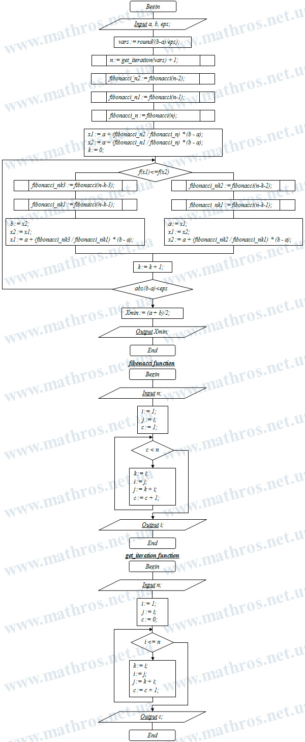
Now look at the flowchart below not only as an illustration, but also as a ready foundation for a small learning project. Why not use it as a clear guide and write a compact program in your favorite programming language that determines the minimum value of a unimodal function using the Fibonacci method? This kind of work clearly shows how theoretical ideas turn into real calculations that you can test on different functions and intervals. In addition, it is a great opportunity to check yourself and understand how confidently you navigate the logic of the method not only in notes and formulas, but also in software implementation.