Inverse of a matrix is often associated with computing a determinant, working with minors, or performing row operations. But is that always the most convenient route? In fact, if the coefficients of a matrix’s characteristic polynomial are already known, we can obtain a formula for the inverse in a fairly direct way.
In this article, we will focus on the main point: how, relying on the Cayley–Hamilton theorem and the coefficients of the characteristic polynomial, we can reach an explicit expression for \( A^{-1} \). And one more important question: why is the coefficient of the constant term so crucial here? Let’s go through it step by step.
Inverse of a Matrix via the Characteristic Polynomial: The Key Transition
Let a nonsingular matrix be given:
\[
A \in \mathbb{R}^{n\times n}, \qquad \det(A)\neq 0.
\]
Its characteristic polynomial is written as:
\[
\det(\lambda \cdot E – A)=\lambda^{n}+p_{1} \cdot \lambda^{n-1}+\cdots+p_{n-1} \cdot \lambda+p_{n},
\]
where \( E \) is the identity matrix of order \( n \), and \( p_{1},p_{2},\ldots,p_{n} \) are the coefficients.
Next, we use the Cayley–Hamilton theorem: the matrix \( A \) is a root of its own characteristic polynomial. So, by substituting \( \lambda=A \), we obtain the zero matrix:
\[
A^{n}+p_{1} \cdot A^{n-1}+\cdots+p_{n-1} \cdot A+p_{n} \cdot E=0.
\]
Now we move to the crucial step. We want a formula for \( A^{-1} \), so we multiply this matrix equation on the left by \( A^{-1} \). This reduces the powers of \( A \) by one and, at the same time, introduces a term containing \( A^{-1} \):
\[
A^{-1} \cdot \Bigl(A^{n}+p_{1} \cdot A^{n-1}+\cdots+p_{n-1} \cdot A+p_{n} \cdot E\Bigr)=A^{-1}\cdot 0.
\]
Since \( A^{-1} \cdot A=E \), we get:
\[
A^{n-1}+p_{1} \cdot A^{n-2}+\cdots+p_{n-1} \cdot E+p_{n} \cdot A^{-1}=0.
\]
Inverse of a Matrix as a Polynomial in the Matrix: Formula and Condition
From the previous equality, we can already isolate \( A^{-1} \). Let’s move everything except the term containing \( A^{-1} \) to the right-hand side:
\[
p_{n} \cdot A^{-1}=-(A^{n-1}+p_{1} \cdot A^{n-2}+\cdots+p_{n-1} \cdot E).
\]
Since the matrix is nonsingular, we have \( \det(A)\neq 0 \), which means \( p_n\neq 0 \) as well. You can see this by substituting \( \lambda=0 \) into the characteristic polynomial:
\[
p_n=\det(0\cdot E-A)=\det(-A)=(-1)^n \cdot \det(A).
\]
So dividing by \( p_n \) is completely justified, and we get an explicit formula:
\[
A^{-1}=-\frac{1}{p_{n}} \cdot \Bigl(A^{n-1}+p_{1} \cdot A^{n-2}+\cdots+p_{n-1} \cdot E\Bigr).
\]
Now let’s highlight an important learning idea. The inverse of a matrix can be expressed as a polynomial in \( A \) of degree at most \( n-1 \). In other words, \( A^{-1} \) is a linear combination of the identity matrix and powers of \( A \):
\[
A^{-1}=c_{0} \cdot E+c_{1} \cdot A+c_{2} \cdot A^{2}+\cdots+c_{n-1} \cdot A^{n-1},
\]
where the coefficients \( c_k \) are determined through \( p_1,\dots,p_n \). Convenient, right? We work with what we already have: the powers of \( A \) and the numbers \( p_k \).
What You Need in Practice
To actually use the formula, follow this short algorithm:
- Find the coefficients \( p_{1},\ldots,p_{n} \).
- Compute the powers \( A, A^{2}, \ldots, A^{n-1} \).
- Substitute everything into the formula for \( A^{-1} \) and obtain the result.
In the very first step, it is most reasonable to use the Leverrier method, because it is specifically designed to efficiently obtain the coefficients of the characteristic polynomial. You can explore the theoretical details of this method in a separate material, but here it is enough to remember the main point: when the goal is to quickly and consistently compute \( p_1,\dots,p_n \), the Leverrier method is usually the most rational choice.
Inverse of a Matrix in Practice: From a Step Plan to Computations
Now that the formula is ready, it’s time to see how it works in real problems. In these examples, the goal is not only to reach the final answer but also to feel the flow of the method: what we take from the characteristic polynomial, what we compute for the matrix itself, and what we can plug into the finished expression right away. Ready to test the method in practice?
Example 1. What steps are needed to find the inverse of a \( 3\times 3 \) matrix if the coefficients of its characteristic polynomial are known?
First, we write down the coefficients of the characteristic polynomial and set up the formula for the case \( n=3 \). Next, we compute the required powers up to order \( n-1 \), meaning we find \( A^{2} \). After that, we substitute these values into the formula for \( A^{-1} \). Finally, it is helpful to do a quick check by multiplying \( A\cdot A^{-1} \) to confirm that the result is the identity matrix.
Example 2. Find the inverse of the matrix if the characteristic polynomial is \( \det(\lambda \cdot E-A)=\lambda^{4}-24 \cdot \lambda^{3}+244 \cdot \lambda^{2}-1818 \cdot \lambda+7881 \)
\[
A=
\begin{pmatrix}
5 & -6 & 7 & 1\\
7 & 10 & -9 & 8\\
3 & 3 & 5 & 1\\
-10 & 2 & 3 & 4
\end{pmatrix}.
\]
We compare this polynomial with the standard form
\[
\det(\lambda \cdot E-A) = \lambda^4 + p_1 \cdot \lambda^3 + p_2 \cdot \lambda^2 + p_3 \cdot \lambda + p_4,
\]
and immediately read off the coefficients:
\[
p_1=-24,\qquad p_2=244,\qquad p_3=-1818,\qquad p_4=7881.
\]
Since \( n=4 \), we use the formula
\[
A^{-1}=-\frac{1}{p_4} \cdot \bigl(A^3 + p_1 \cdot A^2 + p_2 \cdot A + p_3 \cdot E \bigr)
=-\frac{1}{7881} \cdot \bigl(A^3 – 24 \cdot A^2 + 244 \cdot A – 1818 \cdot E \bigr).
\]
Here you can clearly see why we need exactly \( A^{2} \) and \( A^{3} \): they appear in the matrix combination for the case \( n=4 \). After the computations, we get:
\[
\begin{aligned}
A^{2} &= A\cdot A=
\begin{pmatrix}
-6 & -67 & 127 & -32\\
-2 & 47 & -62 & 110\\
41 & 29 & 22 & 36\\
-67 & 97 & -61 & 25
\end{pmatrix},\\[6pt]
A^{3} &= A^{2}\cdot A=
\begin{pmatrix}
202 & -317 & 1100 & -543\\
-967 & 516 & -417 & 752\\
114 & 182 & 244 & 439\\
-89 & 1239 & -1572 & 748
\end{pmatrix}.
\end{aligned}
\]
Substituting into the expression from the formula, we obtain:
\[
A^3 – 24 \cdot A^2 + 244 \cdot A – 1818 \cdot E =
\begin{pmatrix}
-252 & -173 & -240 & 469\\
789 & 10 & -1125 & 64\\
-138 & 218 & -882 & -181\\
-921 & -601 & 624 & -694
\end{pmatrix}.
\]
Therefore,
\[
A^{-1}=-\frac{1}{7881} \cdot
\begin{pmatrix}
-252 & -173 & -240 & 469\\
789 & 10 & -1125 & 64\\
-138 & 218 & -882 & -181\\
-921 & -601 & 624 & -694
\end{pmatrix} \approx
\begin{pmatrix}
0.032&0.022&0.030&-0.060 \\
-0.100&-0.001&0.143&-0.008 \\
0.018&-0.028&0.112&0.023 \\
0.117&0.076&-0.079&0.088
\end{pmatrix}.
\]
Example 3. Find the inverse of the matrix
\[
A=
\begin{pmatrix}
1 & 2 & 3 & 4 \\
2 & 1 & 2 & 3 \\
3 & 2 & -1 & 2 \\
4 & 3 & 2 & 1
\end{pmatrix}.
\]
Here we will do the full cycle: first we compute powers of the matrix, then we compute traces, and from them we obtain the coefficients of the characteristic polynomial using the Leverrier method. After that, we apply the standard formula for \( A^{-1} \). In this kind of problem, the Leverrier method is the best choice, because it allows us to find \( p_{1},\dots,p_{n} \) through the traces \( \operatorname{tr}(A^{k}) \)—and we compute these traces anyway while working with powers of the matrix.
Let’s start with the powers:
\[
\begin{aligned}
A^{2} &= A\cdot A =
\begin{pmatrix}
30 & 22 & 12 & 20 \\
22 & 18 & 12 & 18 \\
12 & 12 & 18 & 18 \\
20 & 18 & 18 & 30
\end{pmatrix},\\[6pt]
A^{3} &= A^{2}\cdot A =
\begin{pmatrix}
190 & 166 & 162 & 230 \\
166 & 140 & 126 & 184 \\
162 & 126 & 78 & 138 \\
230 & 184 & 138 & 200
\end{pmatrix},\\[6pt]
A^{4} &= A^{3}\cdot A =
\begin{pmatrix}
1928 & 1560 & 1200 & 1812 \\
1560 & 1276 & 1020 & 1520 \\
1200 & 1020 & 936 & 1320 \\
1812 & 1520 & 1320 & 1948
\end{pmatrix}.
\end{aligned}
\]
Next, we compute the traces:
\[
\begin{aligned}
\operatorname{tr}(A) &= 1+1-1+1 = 2,\\
\operatorname{tr}(A^{2}) &= 30+18+18+30 = 96,\\
\operatorname{tr}(A^{3}) &= 190+140+78+200 = 608,\\
\operatorname{tr}(A^{4}) &= 1928+1276+936+1948 = 6088.
\end{aligned}
\]
Now, using the Leverrier formulas, we find the coefficients \( p_k \):
\[
\begin{aligned}
p_{1} &= -\operatorname{tr}(A) = -2,\\[2pt]
p_{2} &= -\frac{1}{2} \cdot \Bigl(\operatorname{tr}(A^{2}) + p_{1}\operatorname{tr}(A)\Bigr)
= -\frac{1}{2} \cdot \bigl(96 – 2\cdot 2\bigr) = -46,\\[2pt]
p_{3} &= -\frac{1}{3} \cdot \Bigl(\operatorname{tr}(A^{3}) + p_{1} \cdot \operatorname{tr}(A^{2}) + p_{2} \cdot \operatorname{tr}(A)\Bigr)
= -\frac{1}{3} \cdot \bigl(608 – 2\cdot 96 – 46\cdot 2\bigr) = -108,\\[2pt]
p_{4} &= -\frac{1}{4} \cdot \Bigl(\operatorname{tr}(A^{4}) + p_{1} \cdot \operatorname{tr}(A^{3}) + p_{2} \cdot \operatorname{tr}(A^{2}) + p_{3} \cdot \operatorname{tr}(A)\Bigr)
= -\frac{1}{4} \cdot \bigl(6088 – 2\cdot 608 – 46\cdot 96 – 108\cdot 2\bigr) = -60.
\end{aligned}
\]
So the characteristic polynomial is:
\[
\det(\lambda \cdot E-A)=\lambda^4 – 2 \cdot \lambda^3 – 46 \cdot \lambda^2 – 108 \cdot \lambda – 60.
\]
Since \( n=4 \), the formula for the inverse matrix is:
\[
A^{-1}=-\frac{1}{p_4} \cdot \bigl(A^3 + p_1 \cdot A^2 + p_2 \cdot A + p_3 \cdot E \bigr)
=-\frac{1}{-60} \cdot \bigl(A^3 – 2 \cdot A^2 – 46 \cdot A – 108 \cdot E \bigr)
=\frac{1}{60} \cdot \bigl(A^3 – 2 \cdot A^2 – 46 \cdot A – 108 \cdot E \bigr).
\]
All that remains is to compute the expression in parentheses:
\[
A^3 – 2 \cdot A^2 – 46 \cdot A – 108 \cdot E=
\begin{pmatrix}
-24 & 30 & 0 & 6\\
30 & -50 & 10 & 10\\
0 & 10 & -20 & 10\\
6 & 10 & 10 & -14
\end{pmatrix}.
\]
Then we get:
\[
A^{-1}=\frac{1}{60}\cdot
\begin{pmatrix}
-24 & 30 & 0 & 6\\
30 & -50 & 10 & 10\\
0 & 10 & -20 & 10\\
6 & 10 & 10 & -14
\end{pmatrix}
\approx
\begin{pmatrix}
-0.400 & 0.500 & 0.000 & 0.100\\
0.500 & -0.833 & 0.167 & 0.167\\
0.000 & 0.167 & -0.333 & 0.167\\
0.100 & 0.167 & 0.167 & -0.233
\end{pmatrix}.
\]
What to Study Next: Topics That Expand Your Toolbox
If you already feel confident working with the characteristic polynomial approach, a natural question comes up: what should you learn next? Below are topics that continue this material in a logical way and add new methods for solving problems you already know.
- Inverse of a Matrix by the Bordering Method: How Adding Rows and Columns Leads to the Result — We will show the main idea of the bordering method and explain how, through step-by-step expansion, you can obtain the inverse matrix.
- Inverse of a Matrix by Block Partitioning: When a Matrix Turns into Convenient Blocks — We will look at the block approach and explain how to invert a matrix by working with its parts.
- Pseudoinverse of a Matrix: Inverting Rectangular and Singular Matrices — We will explain why the pseudoinverse is needed and how it helps in situations where the usual inverse does not exist.
Inverse of a Matrix in Code: Try Building Your Own Mini Calculator
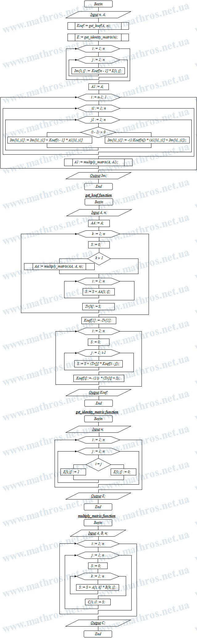
Now imagine that the flowchart below is not just an illustration, but a ready-to-use plan for a small programming project. Why not treat it as a hint and write a short program in your favorite language that computes the inverse of a matrix using the coefficients of the characteristic polynomial?
This kind of task is great for training attention to detail, and at the same time it clearly shows how theory turns into a practical tool you can use again and again. Plus, it’s a nice way to get the result not only “on paper” but also as working code that you can test on your own examples.