Combined Secant-Newton Method: Tangent Speed and Chord Reliability

The combined secant-Newton method blends two strengths of numerical root-finding: it keeps the solution inside a trusted interval and it converges quickly to that solution. We start with an interval that definitely contains a root and, at each step, move its endpoints toward each other: one endpoint is updated by the secant (chord) rule, and the other by the Newton (tangent) rule. This approach works well in both learning examples and real applications because it keeps the process controlled while still moving toward an accurate result at a solid pace.

Combined Secant-Newton Method: Update Choice via the Sign f'(x)⋅f”(x)

Consider the equation f(x)=0 on the initial interval [a₀,b₀]=[a,b] with f(a₀)⋅f(b₀)<0. Assume f is sufficiently smooth on this interval. On each iteration, we update one endpoint by a secant step and the other by a Newton step; which side uses which step is determined by the sign of the product f'(x)⋅f”(x) on the current interval.

If on [an,bn] we have f'(x)⋅f”(x)>0 (cases 1 and 2 in the figure), move the left endpoint with the secant and the right endpoint with Newton:

In this configuration, the Newton step from the right lands inside the interval, while the left secant step steadily trims the interval.

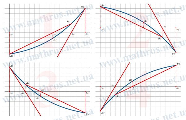
If f'(x)⋅f”(x)<0 (cases 3 and 4), swap the roles: apply the Newton step on the left and the secant on the right:

This choice keeps both new endpoints inside [a_n,b_n] and makes the interval length decrease monotonically. The sign of f'(x)⋅f”(x) tells us from which side Newton’s step remains inside the interval, while the secant step ensures stable shrinking from the opposite side.

Convergence and Accuracy Control: Stopping Rule and Practical Safeguards

It’s convenient to stop the iterations when the current interval becomes smaller than a preset tolerance ε, that is, when (b_n-a_n)<ε. As an approximation to the root, we often take the midpoint of the interval:

in which case the absolute error does not exceed (b_n-a_n)/2. This criterion is easy to implement and immediately gives a clear estimate of result quality without extra checks.

A few practical tips improve efficiency:

• In the secant update, fix one point at the endpoint that was just refreshed by a Newton step from the opposite side. The secant through the “fresh” estimate and the other endpoint usually shortens the interval noticeably.
• Ensure the derivative f'(x) at the Newton step node is not too small. If the denominator makes the update unstable, reduce the step size or temporarily replace the Newton step with a secant update.
• For reliability, choose the initial interval within a region of constant convexity/concavity and without a sign change of f’ near the root. Under these conditions the step-side choice stays correct, and convergence is predictable.

Practical Worked Example: Combined Secant-Newton Method in Action

Now that we’ve covered the basics, let’s see how the combined secant-Newton method behaves on a concrete example. Theory sets the stage; practice shows how those steps turn into an accurate numerical result. We’ll take a problem from start to finish and track how the method reaches the answer with the required precision.

Example 1. Find, with accuracy ε=0.01, the solution of the nonlinear equation f(x)=x³+x-5=0 on the interval [0,2]

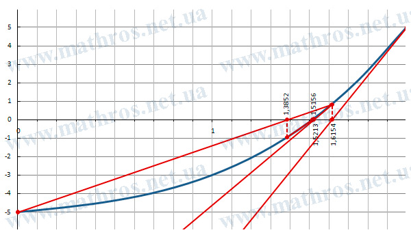
First, check that a root exists: f(0)=-5<0 and f(2)=5>0, so f(x) changes sign on [0,2]. Therefore, there is at least one root in this interval.

On this interval, f'(x)=3⋅x²+1>0 and f”(x)=6⋅x≥0 (positive for x>0). Hence, in the region where the root lies, we have f'(x)⋅f”(x)>0. We follow the combined rule: update the right endpoint with a Newton step and the left endpoint with a secant step, and in the secant formula use the “fresh” right endpoint.

For the right endpoint b₀=2, take one Newton step:

Next, from the left endpoint a₀=0, take a secant step using the points a₀ and the updated b₁:

After this, we have [a₁,b₁]=[1.3852,1.6154] with f(a₁)=-0.9569 and f(b₁)=0.8308.

On the new interval, repeat the same scheme. First, update the right endpoint:

Now update the left endpoint by a secant step using a₁ and the “fresh” b₂:

We obtain [a₂,b₂]=[1.5156,1.5213] with length (b₂-a₂)=0.0057<ε. The stopping criterion is satisfied, so we take the midpoint as the approximation:

The guaranteed error bound is (b₂-a₂)/2=0.0028, which is clearly smaller than ε. For reference, the function value at this approximation is f(x)=0.0191, which is consistent with the small width of the final interval. Thus, in just two steps on [0,2], the combined approach delivers the root estimate x=1.5184 with a reliable accuracy guarantee.

Going Deeper: Three Next Steps to New Possibilities

Now that the core ideas are confirmed in practice, expand your toolkit with methods that naturally complement this approach:

1. Bisection Method: A Controlled Path to the Root — A reliable way to shrink the interval while keeping the solution inside it; a good choice when you need stability and a simple implementation.
2. Method of Successive Approximations: Turn the Equation into an Iterative Process — Build the solution step by step using a simple functional iteration with clear convergence conditions.
3. Interpolation-based Approaches: Approximating the Function to Locate the Exact Root — Replace a complex function with a manageable approximation and solve for the root of the interpolant.

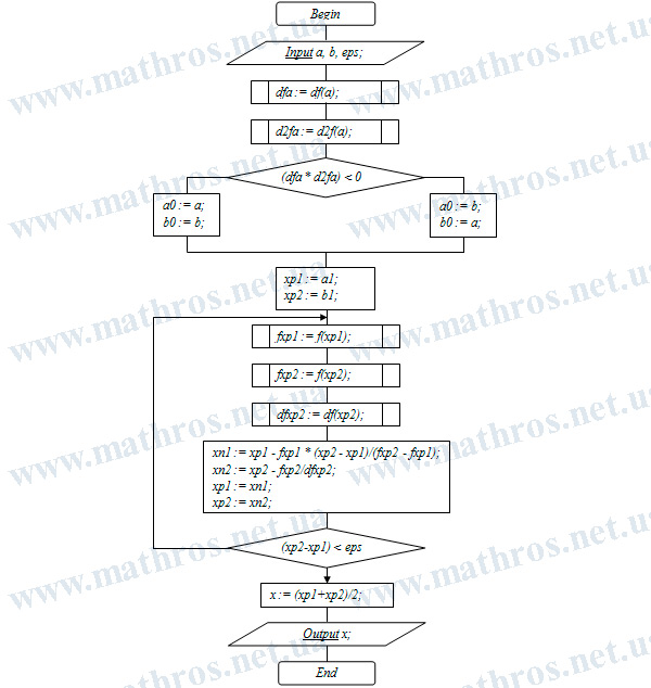
Final Step: Turning the Flowchart into a Program

If you enjoy programming, translate the flowchart into a small learning program and see how the combined secant-Newton method behaves in a real run. Isn’t it satisfying when a visual logic leads to a concrete numerical result and confirms your expectations? Choose a convenient environment, implement the sequence from the diagram, and watch the approximations close in—feel the pace and control. Try several starting intervals, compare behavior across examples, and your confidence will grow. This hands-on practice reinforces knowledge, shows practical value, and makes the path from theory to results direct and understandable.