The Gauss forward and backward interpolation formulas are used to approximate function values at equally spaced nodes when the given point lies near the central part of the table. Unlike Newton’s forward and backward interpolation formulas for equally spaced nodes, which are convenient to use near the beginning or end of a table, Gauss formulas construct the approximation around a central node. We will look at how both formulas are constructed, how to choose between them, and then reinforce what we have learned with practical examples.
Equally Spaced Nodes: Setting Up the Central Interpolation Problem
Suppose we are given \( 2\cdot n+1 \) equally spaced interpolation nodes
\[ x_{-n},x_{-(n-1)},\dots,x_{-1},x_0,x_1,\dots,x_{n-1},x_n, \]
where the distance between neighboring nodes is
\[ x_{i+1}-x_i=h, \qquad i=-n,-(n-1),\dots,n-1. \]
We will consider \( x_0 \) to be the central node. Since the step \( h \) is constant, the coordinates of all other nodes can be expressed in terms of it:
\[ x_i=x_0+i\cdot h. \]
Suppose that for the function \( y=f(x) \), its values are known:
\[ y_i=f(x_i), \qquad i=0,\pm1,\pm2,\dots,\pm n. \]
We need to construct an interpolation polynomial \( P(x) \) of degree at most \( 2\cdot n \) that takes the same values as the function at the given nodes:
\[ P(x_i)=y_i, \qquad i=0,\pm1,\pm2,\dots,\pm n. \]
For the next step, it is convenient to replace the coordinate \( x \) with a quantity that shows the position of the point relative to the central node in units of the step \( h \).
Central Node: Moving to a Dimensionless Argument
Let us introduce the variable
\[ q=\frac{x-x_0}{h}. \]
Hence,
\[ x=x_0+q\cdot h. \]
For any node, we have
\[ x_i=x_0+i\cdot h, \]
so
\[ x-x_i=(q-i)\cdot h. \]
With this substitution, products of differences between \( x \) and the interpolation nodes can be written using simple factors
\[ q,\qquad q-1,\qquad q+1,\qquad q-2,\qquad q+2,\dots. \]
The parameter \( q \) shows how far the point \( x \) is from the central node \( x_0 \) when the distance is measured in steps of \( h \). For a point close to \( x_0 \), the absolute value of \( q \) will be small.
The next step is to construct finite differences, which are used to form the terms of the Gauss interpolation formulas.
Gauss Forward and Backward Interpolation Formulas: Finite Difference Table
For equally spaced nodes, the first finite differences are defined as
\[ \Delta y_i=y_{i+1}-y_i. \]
The second differences are obtained from the first ones:
\[ \Delta^2y_i=\Delta y_{i+1}-\Delta y_i. \]
Similarly, a difference of any order is calculated using the formula
\[ \Delta^ky_i = \Delta^{k-1}y_{i+1} – \Delta^{k-1}y_i. \]
By successively calculating the first, second, and higher-order differences, we obtain a finite difference table.
The Gauss formulas use specific sequences of entries from this table located near its central part.
For the forward formula, we select
\[ \Delta y_0,\quad \Delta^2y_{-1},\quad \Delta^3y_{-1},\quad \Delta^4y_{-2},\quad \Delta^5y_{-2},\quad \Delta^6y_{-3},\dots. \]
For the backward formula, the sequence is
\[ \Delta y_{-1},\quad \Delta^2y_{-1},\quad \Delta^3y_{-2},\quad \Delta^4y_{-2},\quad \Delta^5y_{-3},\quad \Delta^6y_{-3},\dots. \]
If these elements are marked directly in the table, they form two zigzag lines. One corresponds to the Gauss forward interpolation formula, while the other corresponds to the Gauss backward interpolation formula. This representation makes it easy to see exactly which finite differences should be used.
| \( i \) | \( y_i \) | \( \Delta y_i \) | \( \Delta^2 y_i \) | \( \Delta^3 y_i \) | \( \Delta^4 y_i \) | \( \Delta^5 y_i \) | \( \Delta^6 y_i \) |
|---|---|---|---|---|---|---|---|
| \( -3 \) | \( y_{-3} \) | \( \Delta y_{-3} \) | \( \Delta^2 y_{-3} \) | \( \Delta^3 y_{-3} \) | \( \Delta^4 y_{-3} \) | \( \Delta^5 y_{-3} \) | \( \Delta^6 y_{-3} \) |
| \( -2 \) | \( y_{-2} \) | \( \Delta y_{-2} \) | \( \Delta^2 y_{-2} \) | \( \Delta^3 y_{-2} \) | \( \Delta^4 y_{-2} \) | \( \Delta^5 y_{-2} \) | |
| \( -1 \) | \( y_{-1} \) | \( \Delta y_{-1} \) | \( \Delta^2 y_{-1} \) | \( \Delta^3 y_{-1} \) | |||
| \( 0 \) | \( y_0 \) | \( \Delta y_0 \) | \( \Delta^2 y_0 \) | ||||
| \( 1 \) | \( y_1 \) | \( \Delta y_1 \) | |||||
| \( 2 \) | \( y_2 \) | \( \Delta y_2 \) | |||||
| \( 3 \) | \( y_3 \) |
The central nature of these formulas comes from the fact that the required differences are selected near the central node \( x_0 \).
Gauss Forward Interpolation Formula: Construction Using the Lower Difference Scheme
For the Gauss forward interpolation formula, the nodes are included in the construction of the polynomial in the following order:
\[ x_0,\quad x_1,\quad x_{-1},\quad x_2,\quad x_{-2},\dots. \]
First, we take the central node, then the nearest node to its right, followed by the nearest node to its left. We then move progressively farther from the central node.
With this ordering of the nodes, the initial part of the interpolation polynomial has the form
\[ \begin{gathered} P(x)=a_0+a_1\cdot(x-x_0)+a_2\cdot(x-x_0)\cdot(x-x_1)\\[4pt] +a_3\cdot(x-x_{-1})\cdot(x-x_0)\cdot(x-x_1)+\dots. \end{gathered} \]
The coefficients are determined using finite differences. The first few coefficients are
\[ \begin{gathered} a_0=y_0,\\[4pt] a_1=\frac{\Delta y_0}{1!\cdot h}, \qquad a_2=\frac{\Delta^2y_{-1}}{2!\cdot h^2},\\[4pt] a_3=\frac{\Delta^3y_{-1}}{3!\cdot h^3}, \qquad a_4=\frac{\Delta^4y_{-2}}{4!\cdot h^4}. \end{gathered} \]
After introducing the variable \( q \), we obtain the Gauss forward interpolation formula:
\[ \begin{gathered} P(x) = y_0 + q\cdot\Delta y_0 + \frac{q\cdot(q-1)}{2!}\cdot\Delta^2y_{-1}\\[4pt] + \frac{(q+1)\cdot q\cdot(q-1)}{3!}\cdot\Delta^3y_{-1} + \frac{(q+1)\cdot q\cdot(q-1)\cdot(q-2)}{4!}\cdot\Delta^4y_{-2}\\[4pt] + \frac{(q+2)\cdot(q+1)\cdot q\cdot(q-1)\cdot(q-2)}{5!}\cdot\Delta^5y_{-2} +\dots. \end{gathered} \]
In each successive term, the order of the finite difference increases by one, and a new factor is added to the corresponding product.
For an odd order \( 2\cdot k-1 \), the corresponding term has the form
\[ \frac{ \prod_{j=-(k-1)}^{k-1}(q-j) }{ (2\cdot k-1)! } \cdot \Delta^{2\cdot k-1}y_{-(k-1)}, \]
and for an even order \( 2\cdot k \),
\[ \frac{ \prod_{j=-(k-1)}^{k}(q-j) }{ (2\cdot k)! } \cdot \Delta^{2\cdot k}y_{-k}. \]
Therefore, the Gauss forward interpolation formula can be written compactly as
\[ P(x) = y_0 + \sum_{k=1}^{n} \left( \frac{ \prod_{j=-(k-1)}^{k-1}(q-j) }{ (2\cdot k-1)! } \cdot \Delta^{2\cdot k-1}y_{-(k-1)} + \frac{ \prod_{j=-(k-1)}^{k}(q-j) }{ (2\cdot k)! } \cdot \Delta^{2\cdot k}y_{-k} \right). \]
Thus, successively adding nodes to the right and left of \( x_0 \) leads to the first form of the central interpolation polynomial.
Gauss Backward Interpolation Formula: Construction Using the Upper Difference Scheme
For the Gauss backward interpolation formula, the order in which the nodes are included changes:
\[ x_0,\quad x_{-1},\quad x_1,\quad x_{-2},\quad x_2,\dots. \]
Now, after the central node, the nearest node to the left is used first. Because of this, the indices of the finite differences and the structure of the factors for even orders change.
After introducing the variable \( q \), the Gauss backward interpolation formula takes the form
\[ \begin{gathered} P(x) = y_0 + q\cdot\Delta y_{-1} + \frac{(q+1)\cdot q}{2!}\cdot\Delta^2y_{-1}\\[4pt] + \frac{(q+1)\cdot q\cdot(q-1)}{3!}\cdot\Delta^3y_{-2} + \frac{(q+2)\cdot(q+1)\cdot q\cdot(q-1)}{4!}\cdot\Delta^4y_{-2}\\[4pt] + \frac{(q+2)\cdot(q+1)\cdot q\cdot(q-1)\cdot(q-2)}{5!}\cdot\Delta^5y_{-3} +\dots. \end{gathered} \]
For an odd order \( 2\cdot k-1 \), the corresponding term is written as
\[ \frac{ \prod_{j=-(k-1)}^{k-1}(q-j) }{ (2\cdot k-1)! } \cdot \Delta^{2\cdot k-1}y_{-k}, \]
and for an even order \( 2\cdot k \),
\[ \frac{ \prod_{j=-k}^{k-1}(q-j) }{ (2\cdot k)! } \cdot \Delta^{2\cdot k}y_{-k}. \]
In general, the Gauss backward interpolation formula has the form
\[ P(x) = y_0 + \sum_{k=1}^{n} \left( \frac{ \prod_{j=-(k-1)}^{k-1}(q-j) }{ (2\cdot k-1)! } \cdot \Delta^{2\cdot k-1}y_{-k} + \frac{ \prod_{j=-k}^{k-1}(q-j) }{ (2\cdot k)! } \cdot \Delta^{2\cdot k}y_{-k} \right). \]
Thus, the backward formula is constructed according to the same central principle, but it uses a different direction for the first step from \( x_0 \).
Gauss Forward and Backward Interpolation Formulas: Choosing an Approximation Method
Since both formulas are centered around the central node \( x_0 \), the choice between them can conveniently be related to the position of the point \( x \).
If
\[
q>0,
\]
then the point \( x \) lies to the right of \( x_0 \). In this case, it is usually more convenient to use the Gauss forward interpolation formula.
If
\[ q<0, \]
the point lies to the left of the central node, so it is more natural to use the Gauss backward interpolation formula.
Both formulas work best when the absolute value of \( q \) is small, meaning that the point lies close to \( x_0 \). If the point is far from the central part of the selected table, it is better to choose a different central node or use another interpolation formula that is better suited to the location of the point.
If all terms up to order \( 2\cdot n \) are used, the Gauss forward and backward interpolation formulas lead to the same unique interpolation polynomial that passes through all the given nodes. The difference between them lies in how this polynomial is constructed and in the order in which the finite differences are used.
In approximate calculations, only the first few terms of the formula are sometimes used. In that case, the choice between the Gauss forward and backward interpolation formulas can affect the accuracy of the resulting approximation.
Gauss Forward and Backward Interpolation Formulas: Step-by-Step Examples
Let us now move on to the practical use of the Gauss formulas for equally spaced tabulated data. For each problem, we will determine the step size and the central node, construct the required finite differences, find the parameter \( q \), and choose the appropriate formula.
Example 1. Using the given tabulated function values, find the approximate value of \( f(2.4) \)
| \( i \) | \( x_i \) | \( y_i \) |
|---|---|---|
| \( -2 \) | \( 0 \) | \( 1 \) |
| \( -1 \) | \( 1 \) | \( 0 \) |
| \( 0 \) | \( 2 \) | \( 5 \) |
| \( 1 \) | \( 3 \) | \( 22 \) |
| \( 2 \) | \( 4 \) | \( 57 \) |
The distance between neighboring nodes is constant:
\[ h=1. \]
The central node is
\[ x_0=2, \qquad y_0=5. \]
Let us construct the finite difference table:
| \( i \) | \( y_i \) | \( \Delta y_i \) | \( \Delta^2 y_i \) | \( \Delta^3 y_i \) | \( \Delta^4 y_i \) |
|---|---|---|---|---|---|
| \( -2 \) | \( 1 \) | \( -1 \) | \( 6 \) | \( 6 \) | \( 0 \) |
| \( -1 \) | \( 0 \) | \( 5 \) | \( 12 \) | \( 6 \) | |
| \( 0 \) | \( 5 \) | \( 17 \) | \( 18 \) | ||
| \( 1 \) | \( 22 \) | \( 35 \) | |||
| \( 2 \) | \( 57 \) |
Let us calculate the parameter \( q \):
\[ q=\frac{x-x_0}{h} = \frac{2.4-2}{1} = 0.4. \]
Since
\[ q>0, \]
we will use the Gauss forward interpolation formula.
From the table, we select
\[ \Delta y_0=17, \qquad \Delta^2y_{-1}=12, \qquad \Delta^3y_{-1}=6. \]
The fourth difference is zero, so the next term of the formula does not affect the result.
Let us write the required terms of the forward formula:
\[ P(x) = y_0 + q\cdot\Delta y_0 + \frac{q\cdot(q-1)}{2!}\cdot\Delta^2y_{-1} + \frac{(q+1)\cdot q\cdot(q-1)}{3!}\cdot\Delta^3y_{-1}. \]
Substitute the known values:
\[ P(2.4) = 5 + 0.4\cdot17 + \frac{0.4\cdot(0.4-1)}{2}\cdot12 + \frac{(0.4+1)\cdot0.4\cdot(0.4-1)}{6}\cdot6. \]
Now calculate the individual terms:
\[ \begin{gathered} 0.4\cdot17=6.8,\\[4pt] \frac{0.4\cdot(-0.6)}{2}\cdot12=-1.44,\\[4pt] \frac{1.4\cdot0.4\cdot(-0.6)}{6}\cdot6=-0.336. \end{gathered} \]
Therefore,
\[ P(2.4) = 5+6.8-1.44-0.336 = 10.024. \]
Hence,
\[ f(2.4)\approx10.024. \]
Example 2. Using the given tabulated function values, find the approximate value of \( f(-0.6) \)
| \( i \) | \( x_i \) | \( y_i \) |
|---|---|---|
| \( -2 \) | \( -2 \) | \( -8 \) |
| \( -1 \) | \( -1 \) | \( 1 \) |
| \( 0 \) | \( 0 \) | \( 4 \) |
| \( 1 \) | \( 1 \) | \( 7 \) |
| \( 2 \) | \( 2 \) | \( 16 \) |
The step between neighboring nodes is
\[ h=1. \]
The central node is
\[ x_0=0, \qquad y_0=4. \]
Let us calculate the finite differences:
| \( i \) | \( y_i \) | \( \Delta y_i \) | \( \Delta^2 y_i \) | \( \Delta^3 y_i \) | \( \Delta^4 y_i \) |
|---|---|---|---|---|---|
| \( -2 \) | \( -8 \) | \( 9 \) | \( -6 \) | \( 6 \) | \( 0 \) |
| \( -1 \) | \( 1 \) | \( 3 \) | \( 0 \) | \( 6 \) | |
| \( 0 \) | \( 4 \) | \( 3 \) | \( 6 \) | ||
| \( 1 \) | \( 7 \) | \( 9 \) | |||
| \( 2 \) | \( 16 \) |
For the given point,
\[ q=\frac{x-x_0}{h} = \frac{-0.6-0}{1} = -0.6. \]
Since
\[ q<0, \]
we will use the Gauss backward interpolation formula.
From the table, we select
\[ \Delta y_{-1}=3, \qquad \Delta^2y_{-1}=0, \qquad \Delta^3y_{-2}=6. \]
The fourth difference is zero, so it is enough to include the terms up to the third order:
\[ P(x) = y_0 + q\cdot\Delta y_{-1} + \frac{(q+1)\cdot q}{2!}\cdot\Delta^2y_{-1} + \frac{(q+1)\cdot q\cdot(q-1)}{3!}\cdot\Delta^3y_{-2}. \]
Substitute the values:
\[ \begin{gathered} P(-0.6) = 4 + (-0.6)\cdot3 + \frac{(-0.6+1)\cdot(-0.6)}{2}\cdot0\\[4pt] + \frac{(-0.6+1)\cdot(-0.6)\cdot(-0.6-1)}{6}\cdot6. \end{gathered} \]
Now calculate the nonzero terms:
\[ \begin{gathered} (-0.6)\cdot3=-1.8,\\[4pt] \frac{0.4\cdot(-0.6)\cdot(-1.6)}{6}\cdot6=0.384. \end{gathered} \]
Therefore,
\[ P(-0.6) = 4-1.8+0.384 = 2.584. \]
Hence,
\[ f(-0.6)\approx2.584. \]
Example 3. Using the given tabulated function values, find the approximate value of \( f(0.2) \)
| \( i \) | \( x_i \) | \( y_i \) |
|---|---|---|
| \( -2 \) | \( -1 \) | \( 17 \) |
| \( -1 \) | \( -0.5 \) | \( 3 \) |
| \( 0 \) | \( 0 \) | \( 3 \) |
| \( 1 \) | \( 0.5 \) | \( 5 \) |
| \( 2 \) | \( 1 \) | \( 21 \) |
The step between neighboring nodes is
\[ h=0.5. \]
The central node is
\[ x_0=0, \qquad y_0=3. \]
Let us construct the finite difference table:
| \( i \) | \( y_i \) | \( \Delta y_i \) | \( \Delta^2 y_i \) | \( \Delta^3 y_i \) | \( \Delta^4 y_i \) |
|---|---|---|---|---|---|
| \( -2 \) | \( 17 \) | \( -14 \) | \( 14 \) | \( -12 \) | \( 24 \) |
| \( -1 \) | \( 3 \) | \( 0 \) | \( 2 \) | \( 12 \) | |
| \( 0 \) | \( 3 \) | \( 2 \) | \( 14 \) | ||
| \( 1 \) | \( 5 \) | \( 16 \) | |||
| \( 2 \) | \( 21 \) |
Let us find the parameter \( q \):
\[ q=\frac{x-x_0}{h} = \frac{0.2-0}{0.5} = 0.4. \]
Since
\[ q>0, \]
we will use the Gauss forward interpolation formula.
From the table, we select
\[ \Delta y_0=2, \qquad \Delta^2y_{-1}=2, \qquad \Delta^3y_{-1}=12, \qquad \Delta^4y_{-2}=24. \]
Unlike in the first example, the fourth difference is not zero here, so it must also be included.
Substitute all the required values directly into the formula:
\[ \begin{gathered} P(0.2) = 3 + 0.4\cdot2 + \frac{0.4\cdot(0.4-1)}{2}\cdot2\\[4pt] + \frac{(0.4+1)\cdot0.4\cdot(0.4-1)}{6}\cdot12\\[4pt] + \frac{(0.4+1)\cdot0.4\cdot(0.4-1)\cdot(0.4-2)}{24}\cdot24. \end{gathered} \]
Now calculate the terms:
\[ \begin{gathered} 0.4\cdot2=0.8,\\[4pt] \frac{0.4\cdot(-0.6)}{2}\cdot2=-0.24,\\[4pt] \frac{1.4\cdot0.4\cdot(-0.6)}{6}\cdot12=-0.672,\\[4pt] \frac{1.4\cdot0.4\cdot(-0.6)\cdot(-1.6)}{24}\cdot24=0.538. \end{gathered} \]
Therefore,
\[ P(0.2) = 3+0.8-0.24-0.672+0.538 = 3.426. \]
Hence,
\[ f(0.2)\approx3.426. \]
What to Study Next: Useful Topics to Continue With
After studying the Gauss formulas, you can move on to other methods for approximating function values. These topics will help you see how the approach to interpolation changes depending on the arrangement of the nodes, the calculation method, and the properties of the function itself.
- Bessel’s Formula: Interpolation Near the Middle of a Table — Learn how Bessel’s formula uses equally spaced nodes and central differences to calculate function values between neighboring points.
- Aitken’s Scheme: Step-by-Step Refinement of an Interpolated Value — Explore how Aitken’s scheme combines tabulated values step by step and makes it possible to obtain a result without explicitly constructing an interpolation polynomial.
- Trigonometric Interpolation: Approximating Periodic Functions with Trigonometric Polynomials — See how trigonometric polynomials describe periodic data and help calculate function values between known nodes.
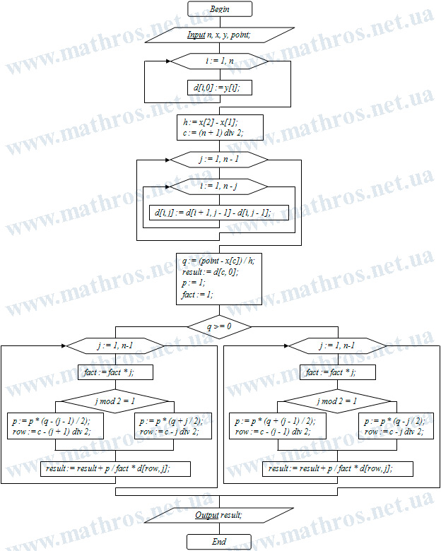
The Two Gauss Interpolation Formulas: From a Flowchart to Your Own Program
If you enjoy programming, try turning the algorithm discussed in this article into your own program. The flowchart below shows the sequence of the main steps: entering the tabulated data, constructing the finite differences, determining the position of the given point, and selecting the appropriate Gauss formula. Implement this algorithm in a programming language you enjoy working with, then test your program using one of the examples from the article and compare the result with the manual calculations.